Electromagnetism: The Principle Map
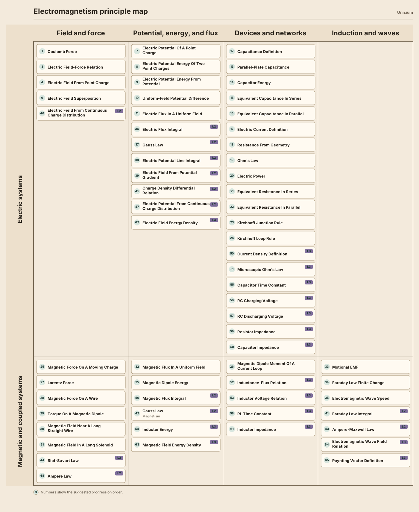
This Electromagnetism guide maps 63 principles using relation families as columns, electric versus magnetic or coupled systems as rows, and three layers: core relations, integral field laws, and dynamic, local, or material models.
Use this reference map to compare field-force, potential-flux-energy, device-network, and induction-wave relations across electric systems and magnetic or coupled systems.
Practice recalling the principles

The Electromagnetism principle map: 63 principles organized by relation family, physical regime, and layer.
On this page
- Why Learn Electromagnetism?
- Prerequisites
- The Principle Map
- Course-Coverage Boundary
- Retrieval Practice
- Core Principles
- What’s Next?
- How This Fits in Unisium
Why Learn Electromagnetism?
Electromagnetism is where physics stops looking like only contact forces and trajectories and starts looking like fields, potentials, flux, and circuit relations. Charges act at a distance through fields. Energy can be tracked through potential difference. Current, resistance, and power become a network story. Magnetic and induction laws add direction, orientation, and field coupling on top of that.
That makes EM structurally different from a formula sheet. The hard part is not just memorizing more equations. It is seeing what kind of physical regime and relation you are dealing with: electric versus magnetic or coupled systems, and within those, whether the step is about field and force, potential and flux, devices and networks, or induction and wave structure. A useful subdomain guide therefore has to do more than list formulas. It has to show how those relations group naturally and form a coherent learning path.
This map covers the core relations of a calculus-based introductory university course, including continuous sources, magnetic dipoles, inductors, transients, AC impedance, field energy, and electromagnetic-wave energy transport. It is a guide to the recurring relations and their conditions, not a claim that the equations replace the geometry, orientation, or physical reasoning needed to solve full problems.
Prerequisites
Mathematics:
- Algebra fluency: rearranging equations, handling proportional relations, and reading reciprocal structure
- Basic vector fluency: magnitude versus vector form, components, dot product, and cross-product direction language
- Comfort with functions and rates, especially for reading field and potential relations
Prior Subdomains:
Calculus note: the map includes field integrals, line and surface orientation, continuous-source geometry, time derivatives, and local material relations. Learners should be comfortable with single-variable calculus and should expect multivariable notation to appear where the physical geometry requires it.
The Principle Map
The map organizes Electromagnetism along two axes:
X-axis (Relation family):
- Field and force - relations that connect charges, currents, fields, and forces
- Potential, energy, and flux - scalar potential structure, potential-energy structure, and field-through-surface relations
- Devices and networks - constitutive and bookkeeping relations for capacitors and lumped circuits
- Induction and waves - later coupled-field relations such as motional EMF and electromagnetic wave speed
Y-axis (Physical regime):
- Electric systems - electrostatics, electric potential and energy, electric flux, capacitors, and circuit-network relations
- Magnetic and coupled systems - magnetic force and field relations, magnetic flux, motional induction, and later wave structure
Layers:
- Core / algebraic - direct algebraic and geometry-constrained EM relations
- Integral and source-geometry field laws - flux integrals, closed-loop and closed-surface laws, field-potential calculus links, density-to-source-element setup, and source-distribution integrals
- Dynamic, local, and material models - time-varying circuit relations, phasor impedance relations, local current-field relations, material-response relations, field-energy relations, and EM-wave energy transport
Progression numbers provide one recommended route through the 63 principles. They do not claim that every course teaches electromagnetism in exactly this order.
The progression is a navigation aid. Use the relation family and physical regime to choose a nearby principle when your course follows a different order.
Why the map uses these axes
The horizontal axis follows the conceptual relation families that recur in electromagnetism. Scan left to right through field and force, potential and flux, devices and networks, and induction and waves. The vertical split then shows whether each relation belongs primarily to electric systems or to magnetic and coupled systems.
Some cells are naturally sparse. Electric systems contribute fewer standalone induction-and-wave relations, while device-and-network relations are more numerous in the electric lane than in the magnetic lane. That imbalance reflects the subject rather than a missing formula list.
The grid is most useful when it helps you distinguish equations that look similar but answer different physical questions. Conditions in the tables make surface choice, loop orientation, source geometry, sign conventions, and circuit regime explicit.
Course-Coverage Boundary
The principle map is broad enough to represent the core relations of a serious calculus-based introductory university electromagnetism course, often called Physics II or introductory E&M.
It includes normal late-intro material: continuous charge sources, Ampere-law magnetostatics, inductors, RC/RL transients, AC impedance, magnetic dipoles and current-loop torque, field energy, EM waves, and the Poynting vector.
It intentionally does not include the upper-division or honors field-theory sequence: differential Maxwell forms, Poisson and Laplace electrostatics, vector potential and gauge material, richer polarization and magnetization theory, transmission lines, waveguides, radiation theory, or full engineering electromagnetics. More advanced courses cover those topics, but they are not required for a strong introductory university E&M foundation.
Practice recalling the principles
This flashcard tool helps make the 63 Electromagnetism principles stronger and easier to access from memory. You practice recalling each principle’s equation or relation and its conditions before revealing the answer.
Use it if you often recognize an electromagnetism equation after seeing it, but struggle to choose between similar field, potential, flux, circuit, or induction relations. Start with core electric-system principles, then add magnetic and coupled systems or later layers when you want a broader review.
Why this works
This tool is based on Vegard Gjerde’s research on structured retrieval practice of physics principle structures. Across this line of work, students practiced retrieving named principles, equations, and conditions instead of only reviewing the completed principle structure. The broader strategy is explained in the Retrieval Practice guide.
Key papers:
- Gjerde, Holst, & Kolstø (2020). Retrieval practice of a hierarchical principle structure in university introductory physics: Making stronger students. Physical Review Physics Education Research, 16(1), 013103.
- Gjerde, Havre Paulsen, Holst, & Kolstø (2022). Problem solving in basic physics: Effective self-explanations based on four elements with support from retrieval practice. Physical Review Physics Education Research, 18(1), 010136.
- Gjerde, Marisaldi, Oksavik, Olafsson, Spångberg, & Holst (2025). Mandatory retrieval test to incentivize retrieval practice of physics principles. Physical Review Physics Education Research, 21(1), 010119.
Equation/form
Conditions
No principles match those filters. Choose at least one relation family, physical regime, and layer.
Core Principles
The tables contain all 63 principles in the map.
Conditions tell you when a principle applies. They are intentionally concise here. Think of them as the discriminating assumptions that separate a valid EM relation from a tempting misuse.
Layer 2 or layer 3 does not mean less important. The layers distinguish the mathematical and physical demands around a relation, not a simple difficulty ranking.
Electric Systems: Field and Force
| Principle | Equation | Condition |
|---|---|---|
| Coulomb Force | point charges; electrostatic; single medium; | |
| Electric Field-Force Relation | nonzero charge when solving for field; field evaluated at a point | |
| Electric Field From Point Charge | point charge; electrostatic; single medium; | |
| Electric Field Superposition | multiple sources; linear superposition regime | |
| Electric Field From Continuous Charge Distribution | continuous charge distribution; field point and source geometry defined |
This is the natural starting point because the relations are direct even when geometry still creates problem difficulty. Coulomb Force and Electric Field From Point Charge use one magnitude equation in the table while their guides also explain the corresponding vector representation.
Electric Systems: Potential, Energy, and Flux
| Principle | Equation | Condition |
|---|---|---|
| Electric Potential Of A Point Charge | point charge; electrostatic; ; reference fixed | |
| Electric Potential Energy Of Two Point Charges | point charges; electrostatic; ; reference fixed | |
| Electric Potential Energy From Potential | charge in a region with defined potential difference | |
| Uniform-Field Potential Difference | uniform field; signed displacement along field axis | |
| Electric Flux In A Uniform Field | uniform field over surface; area vector defined | |
| Electric Flux Integral | surface and area orientation defined | |
| Gauss Law | closed surface; enclosed charge defined; outward orientation | |
| Electric Potential Line Integral | path endpoints and direction fixed; electrostatic field | |
| Electric Field From Potential Gradient | differentiable potential field; coordinates fixed | |
| Charge Density Differential Relation | continuous charge model; density type and source element chosen | |
| Electric Potential From Continuous Charge Distribution | continuous charge distribution; field point and source geometry fixed | |
| Electric Field Energy Density | electric field magnitude defined; linear medium or vacuum permittivity chosen |
This row is broader than scalar potential alone on purpose. It groups the relations that connect field description to scalar energy and surface-through-field structure. For the integral relations, surface choice and path or area orientation are part of applying the equation correctly.
Electric Systems: Devices and Networks
| Principle | Equation | Condition |
|---|---|---|
| Capacitance Definition | lumped-capacitance model | |
| Parallel-Plate Capacitance | parallel plates; negligible fringing; uniform medium | |
| Capacitor Energy | capacitor with defined and | |
| Equivalent Capacitance In Series | series topology already identified | |
| Equivalent Capacitance In Parallel | parallel topology already identified | |
| Electric Current Definition | charge flow through a surface; time interval defined | |
| Resistance From Geometry | uniform conductor; length and cross-section defined | |
| Ohm’s Law | ohmic element; lumped-circuit model; transient operation allowed | |
| Electric Power | lumped element; current and potential difference defined | |
| Equivalent Resistance In Series | series topology already identified | |
| Equivalent Resistance In Parallel | parallel topology already identified | |
| Kirchhoff Junction Rule | lumped-circuit model; steady current bookkeeping | |
| Kirchhoff Loop Rule | closed loop chosen; sign convention fixed | |
| Current Density Definition | current distribution and oriented surface defined | |
| Microscopic Ohm’s Law | ohmic material; local field and conductivity defined | |
| Capacitor Time Constant | first-order RC circuit; effective resistance and capacitance identified | |
| RC Charging Voltage | series RC step charging; | |
| RC Discharging Voltage | series RC discharge path; initial capacitor voltage specified | |
| Resistor Impedance | sinusoidal steady-state; phasor convention and defined | |
| Capacitor Impedance | sinusoidal steady-state; phasor convention// defined |
This combined cell is much more honest than separate capacitor and circuit columns. It gathers the device and network relations that students use once EM stops being only field-at-a-point reasoning and starts becoming component and loop bookkeeping. It also makes the real tension visible: the relations are honest, but topology recognition and sign bookkeeping still live upstream of several of them.
Magnetic and Coupled Systems: Field and Force
| Principle | Equation | Condition |
|---|---|---|
| Magnetic Force On A Moving Charge | moving charge in a magnetic field | |
| Lorentz Force | charge in defined electric and magnetic fields | |
| Magnetic Force On A Wire | straight current-carrying segment in a magnetic field | |
| Magnetic Field Near A Long Straight Wire | long straight wire; steady current; point outside wire | |
| Magnetic Field In A Long Solenoid | long solenoid; interior field approximation | |
| Biot-Savart Law | steady current distribution; source geometry defined | |
| Ampere Law | magnetostatic regime; closed loop; enclosed current defined | |
| Torque On A Magnetic Dipole | magnetic dipole in a magnetic field; orientation defined |
This cell is the magnetic analog of the electric field-and-force group. It connects force laws for moving charges and current-carrying wires with the magnetic-field relations that commonly feed them. The vector equations keep direction visible, while the familiar magnitude forms remain useful when the geometry is already understood. Lorentz Force combines electric and magnetic effects, while Biot-Savart Law connects a current distribution to its magnetic field and therefore depends strongly on geometry.
Magnetic and Coupled Systems: Potential, Energy, and Flux
| Principle | Equation | Condition |
|---|---|---|
| Magnetic Flux In A Uniform Field | uniform field over surface; area vector defined | |
| Magnetic Flux Integral | surface and area orientation defined | |
| Gauss Law For Magnetism | closed surface; outward area orientation | |
| Inductor Energy | inductor model with defined inductance and current | |
| Magnetic Field Energy Density | magnetic field magnitude defined; linear medium or vacuum permeability chosen | |
| Magnetic Dipole Energy | magnetic dipole in uniform external field; reference fixed |
This cell is smaller in the core layer, but the field-calculus layer names the natural magnetic-flux and no-monopole relations explicitly. Surface orientation remains essential when applying them.
Magnetic and Coupled Systems: Devices and Networks
| Principle | Equation | Condition |
|---|---|---|
| Inductance-Flux Relation | inductor or coil model; flux linkage and current defined | |
| Inductor Voltage Relation | inductor model; passive sign convention fixed | |
| RL Time Constant | first-order RL circuit; effective resistance and inductance identified | |
| Inductor Impedance | sinusoidal steady-state; phasor convention// defined | |
| Magnetic Dipole Moment Of A Current Loop | planar current loop; turns/current/area vector defined |
This magnetic device lane includes inductors, RL time scales, AC inductor impedance, and current-loop dipole moment. Sign convention, area-vector orientation, and transient-circuit framing determine which form applies.
Magnetic and Coupled Systems: Induction and Waves
| Principle | Equation | Condition |
|---|---|---|
| Motional EMF | standard motional-EMF geometry; perpendicular motion resolved | |
| Faraday Law Finite Change | loop orientation fixed; average over time interval | |
| Electromagnetic Wave Speed | vacuum-wave context | |
| Faraday Law Integral | closed loop; loop orientation fixed | |
| Ampere-Maxwell Law | closed loop; enclosed current and electric-flux change defined | |
| Electromagnetic Wave Field Relation | plane electromagnetic wave; same point and time | |
| Poynting Vector Definition | co-located fields; linear medium convention fixed |
This group makes the induction and Maxwell bridge explicit. It also highlights decisions that the equation alone cannot make: loop orientation, sign conventions, enclosed-current choices, and the interpretation of changing flux.
Where to Go Next
Use the linked principle guides to move from the map to worked examples and retrieval practice. A practical sequence is:
- Start with Electric Systems: Field and Force to establish the charge-force-field lane.
- Move to Electric Systems: Potential, Energy, and Flux so scalar and surface relations sit next to the earlier field picture.
- Treat Electric Systems: Devices and Networks as the first component and circuit lane rather than as isolated textbook fragments.
- Use the magnetic and coupled-system rows once cross products, magnetic flux, and induction enter the picture.
Later expansion lanes outside this introductory map:
- differential Maxwell forms, Poisson/Laplace electrostatics, vector potential, advanced media, transmission lines, waveguides, radiation theory, and other field-theory or engineering-electromagnetics relations
How This Fits in Unisium
This map connects each principle to the broader electromagnetism structure. It keeps direction rules, symmetry choices, topology recognition, and multi-step problem strategies visible alongside the equations. Use the map to locate the relation you need, then use its guide to learn the conditions, representations, examples, and common failure modes.
Masterful Learning
The book behind these guides: a study system for physics, math, & programming built on retrieval, connection, explanation, and problem solving.
Ready to apply this strategy?
Unisium turns these evidence-based techniques into guided study sessions for math and physics. Places are limited during early access. Check current availability to start a trial; joining the mailing list is optional.
See plans and availability Read More GuidesAlready have access? Sign in