Electric Field Superposition: Add Source Fields As Vectors

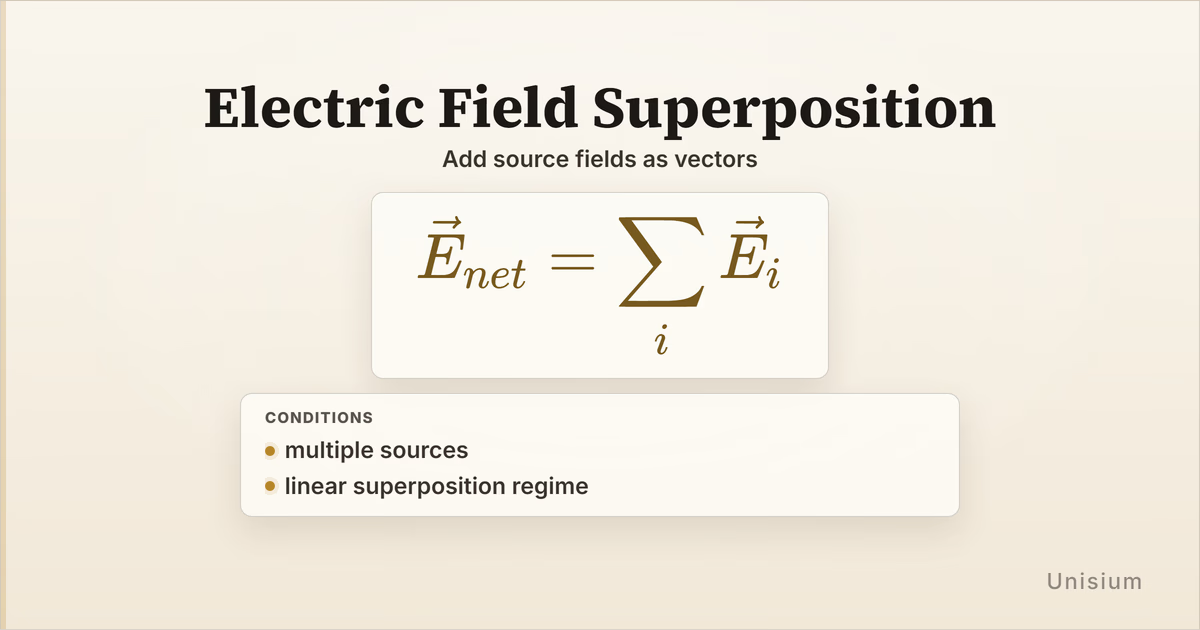
Electric Field Superposition does not replace the one-source laws that build each contribution. It combines those contributions after each relevant source field has been evaluated at the same field point. In early electrostatics that often means using Electric Field From Point Charge first, then summing the resulting vectors.

In ordinary introductory electrostatics in air or vacuum, this linear-addition rule is normally assumed unless the problem says the material response is nonlinear.

The important boundary is between the principle and the surrounding decisions. Superposition says to add the field vectors. It does not decide for you whether a component method, a symmetry argument, or a simple one-dimensional signed axis is the cleanest route for the particular geometry.

On this page: The Principle | Conditions | Misconceptions | Elaborative Encoding | Retrieval Practice | Worked Example | Solve a Problem | Related Principles | FAQ | Related Guides | How This Fits

---

The Principle

Statement

Electric Field Superposition gives the total electric field at a chosen field point by adding the field contributions from all relevant sources as vectors. Each source contributes its own field according to the appropriate source-side law, and the net field is the vector sum of those contributions. When geometry is constrained, the same principle is often carried out through components or symmetry-reduced sums instead of free-form vector addition.

Mathematical Form

$\vec{E}_{net} = \sum_i \vec{E}_i$

Accepted Forms

Component form in a two-dimensional coordinate choice:

$E_{net,x} = \sum_i E_{ix}, \qquad E_{net,y} = \sum_i E_{iy}$

Where:

• $\vec{E}_{net}$ is the net electric field at the field point in $\mathrm{N/C}$
• $\vec{E}_i$ is the electric field contribution from source $i$ at that same field point in $\mathrm{N/C}$
• $E_{net,x}$ and $E_{net,y}$ are the components of the net field in chosen axes
• $E_{ix}$ and $E_{iy}$ are the components of source $i$‘s contribution in those same axes

The diagram keeps one field point fixed and shows two source contributions meeting there. That is the core of the principle: evaluate each source field at the same point, then add those vectors to get the net field.

This particular sketch is symmetric, so the cancellation is easy to see. The principle itself is broader than symmetry. In an unsymmetrical layout you still use the same vector-sum rule, but you no longer get the component cancellation for free.

What this relation does and does not say

• It adds electric fields, not forces, at one chosen field point.
• It keeps direction inside the model step, so non-collinear contributions cannot be combined by magnitude alone.
• It does not replace the source-side relation that gives each individual field contribution.
• It does not force one coordinate choice; components and symmetry are application tools around the same principle.

---

Conditions of Applicability

Condition: multiple sources; linear superposition regime

Practical modeling notes

• Multiple sources means more than one source contributes to the field at the same chosen point.
• Linear superposition regime means the total field is modeled as the sum of the individual source fields without a nonlinear medium response changing that rule.
• Choosing components, symmetry axes, or sign conventions is surrounding setup work, not a separate principle.

When it does not apply directly

This relation fails mainly when the setup cannot be decomposed into separate source contributions that add linearly at one field point.

• Nonlinear medium response: if the medium or model makes the total field differ from the sum of isolated source fields, the linear sum rule is not valid.

Want the complete framework behind this guide? Read Masterful Learning.

---

Common Misconceptions

Misconception 1: Superposition means adding field magnitudes

The truth: Superposition is a vector sum. Magnitudes can be added directly only when every contribution already lies on one signed line.

Why this matters: If you ignore direction, you miss cancellation, reinforcement, and component structure, which are often the whole point of the problem.

Misconception 2: The nearest or largest source automatically determines the net field

The truth: The net field depends on all relevant contributions together with the geometry at the field point.

Why this matters: Many electrostatics mistakes come from dropping a contribution too early and losing the cancellation or reinforcement pattern.

Misconception 3: Superposition replaces the one-source field law

The truth: Superposition combines the individual fields after each one has been modeled. It does not tell you by itself how to compute each $\vec{E}_i$.

Why this matters: Without a source-side model such as Electric Field From Point Charge, the superposition sum has no physical inputs.

---

Elaborative Encoding

Use these questions to build understanding before memorizing the formula. See Elaborative Encoding for the broader method.

Within the Principle

• What stays the same in every term of $\vec{E}_{net} = \sum_i \vec{E}_i$, and what changes from source to source?
• Why is a component sum often safer than a magnitude-only shortcut?

For the Principle

• What clue in a problem tells you that several sources contribute at the same field point, so superposition should enter the model?
• When does symmetry let you predict that one component cancels before you do any arithmetic?

Between Principles

• How is this guide different from Electric Field From Point Charge, which gives one source contribution before superposition combines several?

Generate an Example

• Describe a setup where two nonzero source fields produce a zero net field at one point.

---

Retrieval Practice

Answer from memory, then reveal the result and check it. See Retrieval Practice for the full study method.

State the principle in words: _____The net electric field at a point equals the vector sum of the field contributions from each source evaluated at that same point.

Write the canonical equation: _____$\vec{E}_{net} = \sum_i \vec{E}_i$

State the canonical condition: _____multiple sources; linear superposition regime

---

Worked Example

Use this worked example to practice Self-Explanation.

Problem

Two identical point charges of $q = +2.0\times10^{-6}\,\mathrm{C}$ are fixed at $x = -0.30\,\mathrm{m}$ and $x = +0.30\,\mathrm{m}$. Point $P$ is at $y = 0.40\,\mathrm{m}$ above the midpoint. Find the net electric field vector at $P$ in air. Use $k = 8.99\times10^9\,\mathrm{N\cdot m^2/C^2}$.

Step 1: Verbal Decoding

Target: $\vec{E}_{net}$
Given: $q, x, y, k$
Constraints: multiple sources; linear superposition regime; equal charges; symmetric two-dimensional geometry

Step 2: Visual Decoding

The figure fixes the source geometry: the charges are symmetric about the $y$-axis, and point $P$ lies above the midpoint. Use that symmetry to decide the direction of each source field at $P$, then decide which components cancel or add.

Step 3: Physics Modeling

1. $E_1 = k \frac{q}{(0.50\,\mathrm{m})^2}$
2. $E_2 = k \frac{q}{(0.50\,\mathrm{m})^2}$
3. $E_{net,x} = E_1 \frac{0.30}{0.50} - E_2 \frac{0.30}{0.50}$
4. $E_{net,y} = E_1 \frac{0.40}{0.50} + E_2 \frac{0.40}{0.50}$

Step 4: Mathematical Procedures

1. $E_1 = (8.99\times10^9\,\mathrm{N\cdot m^2/C^2})\frac{2.0\times10^{-6}\,\mathrm{C}}{0.25\,\mathrm{m^2}}$
2. $E_1 = 7.192\times10^4\,\mathrm{N/C}$
3. $E_2 = 7.192\times10^4\,\mathrm{N/C}$
4. $E_{net,x} = (7.192\times10^4\,\mathrm{N/C})\frac{0.30}{0.50} - (7.192\times10^4\,\mathrm{N/C})\frac{0.30}{0.50}$
5. $E_{net,x} = 0$
6. $E_{net,y} = (7.192\times10^4\,\mathrm{N/C})\frac{0.40}{0.50} + (7.192\times10^4\,\mathrm{N/C})\frac{0.40}{0.50}$
7. $E_{net,y} = 1.15072\times10^5\,\mathrm{N/C}$
8. $\underline{\vec{E}_{net} = 1.15\times10^5\,\hat{y}\,\mathrm{N/C}}$

Step 5: Reflection

• Symmetry: Equal positive charges in symmetric positions make the horizontal components cancel exactly.
• Magnitude check: A field on the order of $10^5\,\mathrm{N/C}$ is reasonable for microcoulomb sources only half a meter away.
• Connection to concept: No single source field points straight up, so the upward net field appears only after vector addition.

Before moving on: self-explain the model

Try explaining why superposition is the principle step here, which feature of the sketch guarantees $x$-component cancellation, and why both source fields must be evaluated at the same point before they are added.

Physics model with explanation

Principle: We use Electric Field Superposition because more than one source contributes to the field at the target point.

Conditions: The setup has multiple sources, and the field is modeled in a linear regime where the individual source fields add.

Relevance: This is the right principle when you already know how to build each source contribution and the target is the net field at one location.

Description: Each positive charge creates a field at $P$, and the symmetric geometry turns the vector sum into a clean component cancellation in $x$ and reinforcement in $y$.

Goal: We want the net field vector, not just two separate source fields, so the calculation ends by combining contributions into one final direction and magnitude.

---

Solve a Problem

Apply what you have learned with Problem Solving.

Problem

Two point charges of equal magnitude $q = 2.0\times10^{-6}\,\mathrm{C}$ are fixed at $x = -0.30\,\mathrm{m}$ and $x = +0.30\,\mathrm{m}$. The left charge is positive and the right charge is negative. Point $P$ is at $y = 0.40\,\mathrm{m}$ above the midpoint. Find the net electric field vector at $P$ in air. Use $k = 8.99\times10^9\,\mathrm{N\cdot m^2/C^2}$.

Hint: Determine each source-field direction at $P$ before you add components.

Show Solution

Step 1: Verbal Decoding

Target: $\vec{E}_{net}$
Given: $q, x, y, k$
Constraints: multiple sources; linear superposition regime; equal-magnitude opposite-sign charges; symmetric two-dimensional geometry

Step 2: Visual Decoding

The figure fixes the same symmetric source geometry, but the source signs differ. Determine the direction of each source field at $P$ from the charge signs before adding components.

Step 3: Physics Modeling

1. $E_+ = k \frac{q}{(0.50\,\mathrm{m})^2}$
2. $E_- = k \frac{q}{(0.50\,\mathrm{m})^2}$
3. $E_{net,x} = E_+ \frac{0.30}{0.50} + E_- \frac{0.30}{0.50}$
4. $E_{net,y} = E_+ \frac{0.40}{0.50} - E_- \frac{0.40}{0.50}$

Step 4: Mathematical Procedures

1. $E_+ = (8.99\times10^9\,\mathrm{N\cdot m^2/C^2})\frac{2.0\times10^{-6}\,\mathrm{C}}{0.25\,\mathrm{m^2}}$
2. $E_+ = 7.192\times10^4\,\mathrm{N/C}$
3. $E_- = 7.192\times10^4\,\mathrm{N/C}$
4. $E_{net,x} = (7.192\times10^4\,\mathrm{N/C})\frac{0.30}{0.50} + (7.192\times10^4\,\mathrm{N/C})\frac{0.30}{0.50}$
5. $E_{net,x} = 8.6304\times10^4\,\mathrm{N/C}$
6. $E_{net,y} = (7.192\times10^4\,\mathrm{N/C})\frac{0.40}{0.50} - (7.192\times10^4\,\mathrm{N/C})\frac{0.40}{0.50}$
7. $E_{net,y} = 0$
8. $\underline{\vec{E}_{net} = 8.63\times10^4\,\hat{x}\,\mathrm{N/C}}$

Step 5: Reflection

• Verification: A zero $y$ component and a positive $x$ component match the symmetry of equal magnitudes with opposite charge signs.
• Interpretation: Above this equal-and-opposite pair, the vertical parts cancel while the rightward parts reinforce.
• Parameter dependence: Doubling both charge magnitudes would double the final field magnitude.

---

Related Principles

See Electromagnetism: The Principle Map for placement in the subdomain and the wider guides library for adjacent study paths.

Principle	Relationship to Electric Field Superposition
Electric Field From Point Charge	Gives each one-source field contribution that superposition later combines at one field point.
Coulomb Force	Models force between charges directly, while this guide adds electric-field contributions before any test-charge force step.
Electric Field-Force Relation	After superposition produces the net field, this relation converts that net field into force on a chosen charge.

See Principle Structures for a broader view of how nearby relations connect.

---

FAQ

What is electric field superposition?

It is the rule that the net electric field at a point equals the vector sum of the separate source fields at that same point. The principle matters whenever more than one source contributes to the field.

When can I add electric fields from different charges?

You can add them when the problem has multiple sources and the model is in a linear superposition regime. In ordinary introductory electrostatics, that is the default assumption unless the medium or setup says otherwise.

Do I add magnitudes or vectors in electric field superposition?

You add vectors. Magnitudes can be added directly only in special one-dimensional signed cases where every contribution already lies on the same line.

How is electric field superposition different from electric field from a point charge?

Electric Field From Point Charge gives one source contribution. Electric Field Superposition is the next step that combines several source contributions into one net field.

When should I use components or symmetry in superposition problems?

Use components when contributions are not already collinear, and use symmetry whenever the geometry makes cancellation or reinforcement obvious before the arithmetic. Those are strategy choices around the same vector-sum principle.

When does electric field superposition fail?

It fails when the total field is not modeled as a linear sum of separate source contributions, such as in a nonlinear response where isolated source fields do not simply add.

---

Related Guides

• Electric Field From Point Charge — Build each one-source field before you combine them.
• Electric Field-Force Relation — Turn the resulting net field into force on a charge at the field point.
• Electromagnetism: The Principle Map — Place this relation in the electromagnetism progression.
• Problem Solving — Use superposition inside structured worked examples and solo practice.

---

How This Fits in Unisium

In Unisium, this principle is where one-source electrostatics turns into multi-source field reasoning: first retrieve the vector-sum rule, then explain why geometry decides cancellation or reinforcement, then practice constrained layouts before moving to less symmetric field problems. Check access and join the Unisium waitlist or see the wider framework in Masterful Learning.

Masterful Learning

The book behind these guides: a study system for physics, math, & programming built on retrieval, connection, explanation, and problem solving.

About the book →