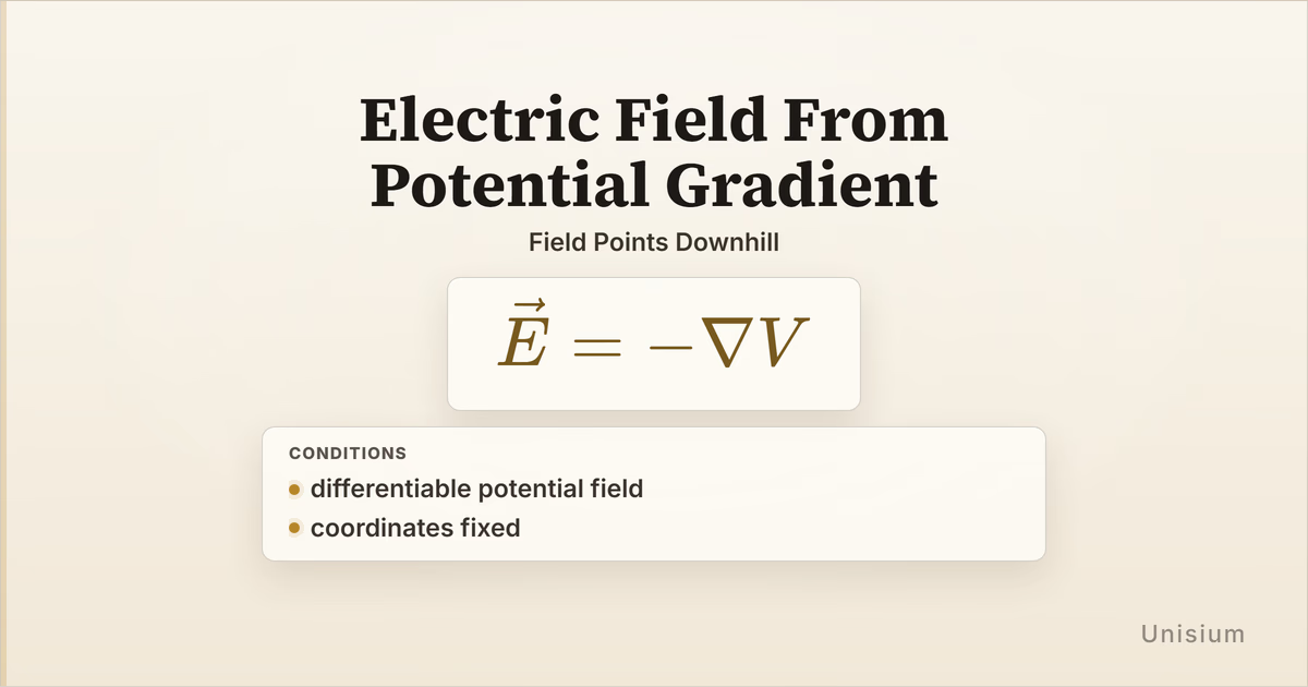
Electric Field From Potential Gradient: Field Points Downhill

This guide reverses the local idea behind Electric Potential Line Integral: instead of accumulating field to get voltage change, it differentiates voltage to get field. The surrounding choices are coordinate axes, contour reading, and component direction; the principle itself is the local field-potential relation.

On this page: The Principle | Conditions | Misconceptions | Elaborative Encoding | Retrieval Practice | Worked Example | Solve a Problem | Related Principles | FAQ | Related Guides | How This Fits

---

The Principle

Statement

Electric Field From Potential Gradient connects a scalar potential field to the local electric field vector. The gradient $\nabla V$ points in the direction where potential increases fastest, and the minus sign says the electric field points toward fastest decrease in potential.

Mathematical Form

$\vec{E} = -\nabla V$

Where:

• $\vec{E}$ is the electric field, in $\mathrm{N/C}$ or $\mathrm{V/m}$
• $V$ is electric potential, in volts
• $\nabla V$ is the spatial gradient of potential in the chosen coordinate system
• The minus sign means field points downhill in potential

In rectangular coordinates, the same relation becomes:

$\vec{E} = -\left(\frac{\partial V}{\partial x}\hat{x}+\frac{\partial V}{\partial y}\hat{y}+\frac{\partial V}{\partial z}\hat{z}\right)$

The coordinate system is part of the setup. The field is a physical vector, but the component calculation depends on the coordinates and unit vectors you have fixed before taking the gradient.

Connection to potential difference

For a small displacement $d\vec{\ell}$, the local change in potential is:

$dV = -\vec{E}\cdot d\vec{\ell}$

That is the local version of Electric Potential Line Integral. The gradient form answers the reverse question: if you already know $V(x,y,z)$, what field must produce those local potential changes?

---

Conditions of Applicability

Condition: differentiable potential field; coordinates fixed

Practical modeling notes

• Differentiable potential field means $V$ changes smoothly enough in the region for spatial derivatives to exist.
• Coordinates fixed means the axes, coordinate variables, and unit-vector basis are already chosen.
• The relation is local: it gives the field at each point from the local spatial rate of change of $V$.
• In one dimension, the relation reduces to $E_x=-dV/dx$ along the chosen axis.

When it does not apply directly

• The potential is not differentiable at the point: use a limiting or piecewise analysis instead of plugging into a local gradient.
• The coordinate basis is not fixed: define the coordinate system before reading gradient components.
• Only an endpoint voltage difference is known: the local gradient form is not directly usable unless you know how $V$ changes in space; use Uniform-Field Potential Difference or the line-integral relation when local field information is missing.

Want the complete framework behind this guide? Read Masterful Learning.

---

Common Misconceptions

Misconception 1: Electric field points toward higher potential

The truth: $\nabla V$ points toward higher potential. The electric field is $-\nabla V$, so it points toward decreasing potential.

Why this matters: Reversing this sign flips the direction of force on a positive test charge.

Misconception 2: A larger potential means a larger field

The truth: The field comes from spatial change in potential, not the absolute value of potential. A constant high potential has zero gradient and therefore zero field.

Why this matters: Field strength depends on slope, not altitude on the potential map.

Misconception 3: Coordinates are a cosmetic detail

The truth: The physical field is coordinate-independent, but the derivative calculation uses the coordinates and unit vectors you choose.

---

Elaborative Encoding

Use these questions to build understanding before memorizing the formula. See Elaborative Encoding for the broader method.

Within the Principle

• Why does the gradient of $V$ point uphill in potential while $\vec{E}$ points downhill?
• What are the units of $\nabla V$, and why do they match electric-field units?

For the Principle

• What wording in a problem tells you the potential field is given as a function of position?
• What coordinate choices must be fixed before you write component derivatives?

Between Principles

• How does this local gradient relation reverse the direction of Electric Potential Line Integral?

Generate an Example

• Describe a potential field that changes with $x$ only, then predict the direction of the electric field.

---

Retrieval Practice

Answer from memory, then reveal the result and check it. See Retrieval Practice for the full study method.

State the principle in words: _____Electric field is the negative gradient of electric potential, so it points in the direction where potential decreases fastest.

Write the canonical equation: _____$\vec{E} = -\nabla V$

State the canonical condition: _____differentiable potential field; coordinates fixed

---

Worked Example

Use this worked example to practice Self-Explanation.

Problem

In a region of space, the electric potential is $V(x,y)=30\,\mathrm{V}-(12\,\mathrm{V/m})x+(5.0\,\mathrm{V/m})y$. Find the electric field vector in the fixed rectangular coordinate system.

Step 1: Verbal Decoding

Target: $\vec{E}$
Given: $V(x,y), x, y$
Constraints: potential field is differentiable; rectangular coordinates are fixed; unit vectors are $\hat{x}$ and $\hat{y}$

Step 2: Visual Decoding

Draw fixed $x$- and $y$-axes, then mark that potential decreases as $x$ increases and increases as $y$ increases. (The key visual fact is that the electric field points toward increasing $x$ and decreasing $y$.)

Step 3: Physics Modeling

1. $E_x = -\frac{\partial V}{\partial x}$
2. $E_y = -\frac{\partial V}{\partial y}$

Step 4: Mathematical Procedures

1. The constant and $y$-only terms have zero $x$ derivative: $E_x = -\frac{\partial}{\partial x}\left[-(12\,\mathrm{V/m})x\right]$
2. The constant and $x$-only terms have zero $y$ derivative: $E_y = -\frac{\partial}{\partial y}\left[(5.0\,\mathrm{V/m})y\right]$
3. $E_x = -(-12\,\mathrm{V/m})$
4. $E_y = -(5.0\,\mathrm{V/m})$
5. $\underline{\vec{E} = (12\,\hat{x}-5.0\,\hat{y})\,\mathrm{V/m}}$

Step 5: Reflection

• Dimensional analysis: A derivative of volts with respect to meters gives $\mathrm{V/m}$, the same as electric field.
• Interpretation: The field has a positive $x$ component because potential decreases as $x$ increases.
• Verification: Moving a small distance in the $+\hat{x}$ direction gives negative $dV$, so $\vec{E}\cdot d\vec{\ell}$ is positive.

Before moving on: self-explain the model

Try explaining why Step 3 uses partial derivatives in the fixed coordinate directions, why the constant $30\,\mathrm{V}$ disappears, and why the minus sign reverses the potential gradient.

Physics model with explanation

Principle: We use Electric Field From Potential Gradient because the problem gives potential as a differentiable function of position and asks for the local field.

Conditions: The potential is differentiable, and the rectangular coordinate axes are fixed before the gradient is taken.

Relevance: The target is the field vector, not an endpoint voltage change, so differentiating the potential is the direct model.

Description: The $x$ derivative measures how potential changes when only $x$ changes; the $y$ derivative does the same for $y$. The electric field is the negative of that gradient.

Goal: Compute the two coordinate derivatives and reverse their signs to get the field components.

---

Solve a Problem

Apply what you have learned with Problem Solving.

Problem

Along the $x$-axis, the electric potential is $V(x)=80\,\mathrm{V}-(40\,\mathrm{V/m})x+(10\,\mathrm{V/m^2})x^2$. Find $E_x$ at $x=1.5\,\mathrm{m}$.

Hint: In one dimension, use $E_x=-dV/dx$ after the coordinate direction is fixed.

Show Solution

Step 1: Verbal Decoding

Target: $E_x$
Given: $V(x), x$
Constraints: potential is differentiable; $x$ coordinate is fixed; field component is requested at one point

Step 2: Visual Decoding

Draw an $x$-axis and mark the point $x=1.5\,\mathrm{m}$. (The key visual fact is that the local slope of $V(x)$ at that point sets the field component with the opposite sign.)

Step 3: Physics Modeling

1. $E_x = -\frac{dV}{dx}\bigg|_{x=1.5\,\mathrm{m}}$

Step 4: Mathematical Procedures

1. $E_x = -\left[-40\,\mathrm{V/m}+(20\,\mathrm{V/m^2})x\right]_{x=1.5\,\mathrm{m}}$
2. $E_x = -\left[-40\,\mathrm{V/m}+(20\,\mathrm{V/m^2})(1.5\,\mathrm{m})\right]$
3. $E_x = -(-10\,\mathrm{V/m})$
4. $\underline{E_x = 10\,\mathrm{V/m}}$

Step 5: Reflection

• Dimensional analysis: The derivative terms both have units of $\mathrm{V/m}$.
• Interpretation: The potential is still decreasing with $x$ at $1.5\,\mathrm{m}$, so the field component is positive.
• Limiting case: At $x=2.0\,\mathrm{m}$, the slope would be zero and the local field component would vanish.

---

Related Principles

See Electromagnetism: The Principle Map for where this gradient relation sits in the field-calculus layer.

Principle	Relationship to Electric Field From Potential Gradient
Electric Potential Line Integral	Accumulates field along a path to get potential difference; the gradient form recovers field locally from potential.
Uniform-Field Potential Difference	The constant-field, one-axis case where potential changes linearly with position.
Electric Potential Of A Point Charge	Gives a source-specific potential that can be differentiated to recover a radial electric field.

See Principle Structures for a broader view of how field and potential relations connect.

---

FAQ

What is Electric Field From Potential Gradient?

Electric Field From Potential Gradient is the relation $\vec{E}=-\nabla V$. It says the electric field equals the negative spatial gradient of electric potential.

Why is there a minus sign in electric field from potential?

The gradient points toward increasing potential. The electric field points toward decreasing potential, so the formula includes a minus sign.

When does this principle apply?

It applies when the potential field is differentiable and the coordinate system is fixed. Those conditions let the spatial derivatives define local field components.

Is electric field the same as potential?

No. Potential is a scalar value at each point, while electric field is a vector that comes from how potential changes with position.

How is this different from the electric potential line integral?

The line integral finds potential difference from a known electric field. The gradient relation goes the other direction: it finds electric field from a known potential function.

---

Related Guides

• Electromagnetism: The Principle Map - Place this relation among potential and field-calculus principles.
• Electric Potential Line Integral - Review the path-integral direction before using the local gradient form.
• Electric Potential Of A Point Charge - Compare a specific potential formula with the general gradient relation.
• Problem Solving - Practice turning givens, conditions, and targets into a usable model.

---

How This Fits in Unisium

Unisium treats Electric Field From Potential Gradient as a principle because a compact equation hides several separable learning moves: fix coordinates, read the potential slope, reverse the gradient direction, and keep absolute potential separate from field strength. The useful learning path is to encode the sign relation, retrieve the condition, self-explain contour and component examples, and solve new problems where the potential function is given.

Ready to master Electric Field From Potential Gradient? Check access and join the Unisium waitlist or explore the full framework in Masterful Learning.

Masterful Learning

The book behind these guides: a study system for physics, math, & programming built on retrieval, connection, explanation, and problem solving.

About the book →