Electric Field From Continuous Charge Distribution: Add dq Fields
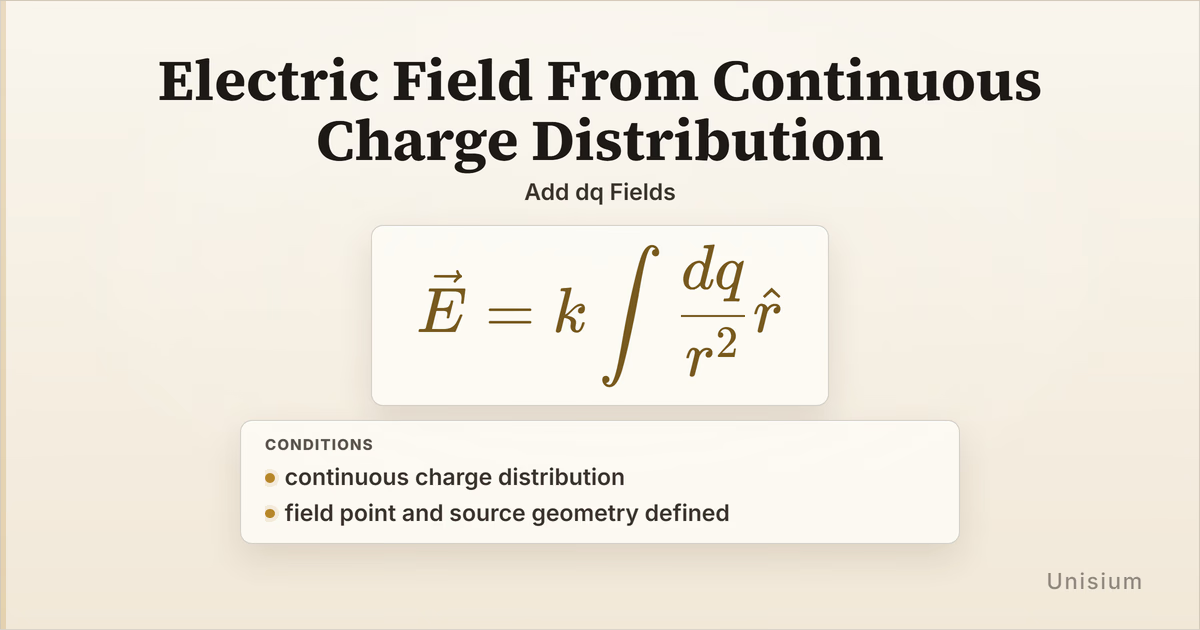
Electric Field From Continuous Charge Distribution gives the electric field made by adding the point-charge field contribution from every small charge element . The model is , and it applies when the charge is continuous and the field point plus source geometry are defined. Use it when a charged object cannot be treated as one point charge.
This guide sits in the field-calculus layer of the Electromagnetism Principle Map, after Charge Density Differential Relation. The surrounding decisions are choosing a source coordinate, writing , defining and from each source element to the field point, and using symmetry or components to make the vector integral manageable. Those decisions support the principle; they are not extra laws to memorize.
On this page: The Principle | Conditions | Misconceptions | Elaborative Encoding | Retrieval Practice | Worked Example | Solve a Problem | Related Principles | FAQ | Related Guides | How This Fits
The Principle
Statement
Electric Field From Continuous Charge Distribution says that a continuous source can be broken into small charge elements, and each element contributes a small electric field at the field point. The total field is the vector integral of those contributions over the source.
Mathematical Form
Where:
- is the total electric field at the field point, in newtons per coulomb
- is Coulomb’s constant for the medium or model, usually in vacuum
- is one small source charge element, in coulombs
- is the distance from that source element to the field point
- points from the source element toward the field point
The diagram is a guide-level source-geometry scaffold. It shows one local source element inside the integral: a small , the source-to-field direction , and the local contribution at point . The full field comes from adding all such contributions, not from treating the whole source as one point charge.
Useful setup forms
The integral becomes usable only after and are tied to the source geometry. For common continuous sources:
- Line source:
- Surface source:
- Volume source:
These are not new electric-field principles. They are source-modeling steps that prepare the same field integral.
Conditions of Applicability
Condition: continuous charge distribution; field point and source geometry defined
Practical modeling notes
- Continuous charge distribution means the source is modeled as charge spread along a line, over a surface, or through a volume.
- Field point defined means the location where is evaluated is fixed before the integral is written.
- Source geometry defined means each source element, distance , direction , and integration boundary can be described.
When it does not apply directly
- Point charges: If the source is a small number of point charges, use Electric Field Superposition with point-charge fields.
- Undefined geometry: If the problem has not fixed the source shape or field point, the integral cannot be set up honestly.
- Symmetry shortcut available: For high-symmetry closed-surface problems, Gauss Law may be the cleaner field relation.
Want the complete framework behind this guide? Read Masterful Learning.
Common Misconceptions
Misconception 1: The whole object acts like one point charge
The truth: A continuous object can be treated as a point charge only under special symmetry or far-away approximation conditions. The integral keeps the changing distance and direction from each source element visible.
Why this matters: Using one distance for the whole object can give the wrong magnitude and direction.
Misconception 2: dq is optional notation
The truth: is the source piece being added. Without connecting to , , or , the integral has no source variable.
Why this matters: Most continuous-source errors start before integration, at the source-element setup.
Misconception 3: The vector direction comes after the integral
The truth: The direction is part of each contribution. Symmetry may cancel components, but those cancellations come from the vector geometry.
Elaborative Encoding
Use these questions to build understanding before memorizing the formula. See Elaborative Encoding for the broader method.
Within the Principle
- What does the factor say about how one source element affects the field point?
- Why is the electric field a vector integral rather than a scalar sum?
For the Principle
- What information must be known before the continuous-source field integral can be written?
- In a line-charge problem, which decisions belong to geometry setup rather than to the principle itself?
Between Principles
- How does Charge Density Differential Relation supply the used in this electric-field integral?
Generate an Example
- Describe one charged object where a continuous-source field integral is more appropriate than a point-charge field formula.
Retrieval Practice
Answer from memory, then reveal the result and check it. See Retrieval Practice for the full study method.
State the principle in words: _____A continuous charge distribution creates electric-field contributions from each small source charge, and the total field is the integral of those contributions over the source.
Write the canonical equation: _____
State the canonical condition: _____continuous charge distribution; field point and source geometry defined
Worked Example
Use this worked example to practice Self-Explanation.
Problem
A uniformly charged thin rod of length lies on the -axis, centered at the origin. Its linear charge density is . Point is on the perpendicular bisector at . Find the electric-field magnitude and direction at .
Step 1: Verbal Decoding
Target: , direction
Given: , , ,
Constraints: continuous line charge; field point on perpendicular bisector; source geometry defined; positive uniform density
Step 2: Visual Decoding
Draw the rod on the -axis from to , place at , mark a source element , and connect it to . (The horizontal components cancel by symmetry, so the field points along .)
Step 3: Physics Modeling
Step 4: Mathematical Procedures
Step 5: Reflection
- Dimensional analysis: has units of times length, and the geometry factor has units of inverse length.
- Interpretation: Symmetry removes the horizontal components, leaving only the vertical field.
- Limiting case: Far from the rod, the expression approaches the point-charge pattern for total charge .
Before moving on: self-explain the model
Try explaining why Step 3 already contains the component, distance function, source element, and symmetry result, and why it does not also list the generic vector integral.
Physics model with explanation
Principle: We use Electric Field From Continuous Charge Distribution because the source is spread over a rod, not concentrated at one point.
Conditions: The charge distribution is continuous, the field point is specified, and the rod geometry fixes the source coordinate and bounds.
Relevance: The target is the electric field at a point, and each contributes a field that must be added over the rod.
Description: A source element at coordinate is distance from . Its vertical contribution includes the factor , and matching elements at and cancel horizontally.
Goal: Sum the vertical contributions from the whole rod and report the remaining field direction.
Solve a Problem
Apply what you have learned with Problem Solving.
Problem
A uniformly charged thin rod of length lies on the -axis, centered at the origin. Its linear charge density is . Point is on the perpendicular bisector at . Find the electric-field magnitude and direction at .
Hint: The perpendicular-bisector symmetry is the same as in the worked example.
Show Solution
Step 1: Verbal Decoding
Target: , direction
Given: , , ,
Constraints: continuous line charge; field point on perpendicular bisector; source geometry defined; positive uniform density
Step 2: Visual Decoding
Draw the rod on the -axis from to , place at , and mark a source element . (The horizontal components cancel, so the field points along .)
Step 3: Physics Modeling
Step 4: Mathematical Procedures
Step 5: Reflection
- Dimensional analysis: The units reduce to newtons per coulomb.
- Interpretation: A positive rod produces a field away from the rod at a point above it.
- Parameter dependence: Increasing would increase the field in direct proportion.
Related Principles
See Electromagnetism: The Principle Map for where this continuous-source field relation sits in the electric field-and-force lane.
- Charge Density Differential Relation: Supplies from a line, surface, or volume density before this field integral is evaluated.
- Electric Field From Point Charge: Gives the local point-charge contribution that this principle integrates over a continuous source.
- Electric Field Superposition: Shares the add-the-contributions idea, but for discrete or separately modeled source fields.
See Principle Structures for a broader way to organize source relations, fields, and symmetry decisions.
FAQ
What is the electric field from a continuous charge distribution?
It is the electric field made by adding the field contribution from every small charge element in a continuous source. The canonical model is .
When does this principle apply?
It applies under the canonical condition: continuous charge distribution; field point and source geometry defined. The source shape, field point, distance function, and source element must be known or inferable.
How is this different from the point-charge electric field?
The point-charge relation uses one source charge and one distance. The continuous-source relation adds many point-charge-like contributions because and can change across the source.
Where does dq come from?
comes from the charge-density model. For a line source, use ; for a surface, use ; for a volume, use .
Does the integral choose the bounds for me?
No. The bounds come from the source geometry and coordinate choice. The principle tells you what contribution to add after the source is represented.
Related Guides
- Electromagnetism: The Principle Map - Place this guide in the field-calculus layer.
- Charge Density Differential Relation - Build the used inside continuous-source integrals.
- Electric Field Superposition - Compare continuous integration with adding discrete source fields.
- Problem Solving - Practice translating a physical setup into equations and constraints.
How This Fits in Unisium
Unisium treats Electric Field From Continuous Charge Distribution as a principle because the equation is compact but the representation work is demanding. The useful learning path is to encode what , , and mean, retrieve the exact condition, self-explain the source geometry, and solve supported problems where the geometry setup is explicit.
Ready to study principles this way? Check access and join the Unisium waitlist or explore the full framework in Masterful Learning.

Masterful Learning
The book behind these guides: a study system for physics, math, & programming built on retrieval, connection, explanation, and problem solving.
Ready to apply this strategy?
Unisium turns these evidence-based techniques into guided study sessions for math and physics. Places are limited during early access. Check current availability to start a trial; joining the mailing list is optional.
See plans and availability Read More GuidesAlready have access? Sign in