Microscopic Ohm's Law: Local Current Density From Electric Field
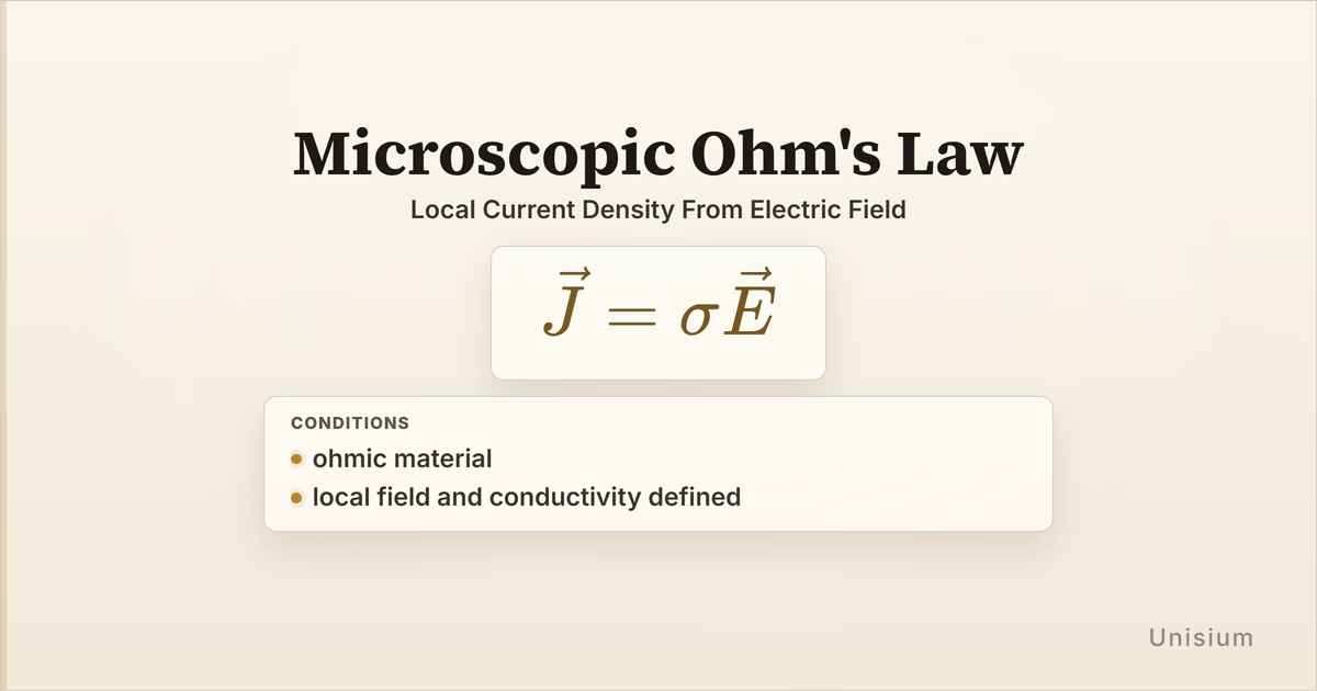
Microscopic Ohm’s Law says local current density is proportional to local electric field in an ohmic material. The model is , and it applies when the material is ohmic and the local field and conductivity are defined. Use it when you need the material response at a point, not the voltage-current relation of a whole circuit element.
This guide connects Current Density Definition to material response and sits beside Ohm’s Law in the Electromagnetism Principle Map. The surrounding decisions are deciding whether the material can be modeled as ohmic, checking that , , and refer to the same local region, and choosing a coordinate direction for component work; those setup choices are not separate principle keys.
On this page: The Principle | Conditions | Misconceptions | Elaborative Encoding | Retrieval Practice | Worked Example | Solve a Problem | Related Principles | FAQ | Related Guides | How This Fits
The Principle
Statement
Microscopic Ohm’s Law models how an ohmic material responds locally to an electric field. Conductivity is the proportionality between the local electric field and the resulting current density . The relation is local: it describes what happens at a point or small region of material before geometry is turned into total current or resistance.
Mathematical Form
Where:
- is current density, in amperes per square meter
- is electrical conductivity, in siemens per meter
- is electric field, in volts per meter
For an isotropic ohmic material, points in the same direction as when is positive. In component form along one chosen axis, the same relation becomes
This component form is not a new principle. It is the same local material relation after you choose an axis.
Connection to macroscopic circuit laws
Microscopic Ohm’s Law is the local version of ohmic behavior. If the material is uniform and the geometry is simple, combining this local relation with Resistance From Geometry prepares the familiar circuit relation . The guide boundary matters: is about local fields inside material, while is about one selected circuit element.
Conditions of Applicability
Condition: ohmic material; local field and conductivity defined
Practical modeling notes
- Ohmic material means the current density is proportional to electric field over the range being modeled.
- Local field and conductivity defined means and are known or modeled at the same point or small region where you want .
- If conductivity varies with position, the relation can still be local, but you must use the local value .
- For anisotropic materials, conductivity can depend on direction. Then the compact scalar form may need a tensor form rather than one number .
When it does not apply directly
- Non-ohmic material: if the current density is not proportional to electric field, one constant conductivity does not describe the response.
- Missing local field: a voltage difference across a whole object is not the same as a known local electric field unless the field model has been established.
- Geometry-only question: if the problem asks for total resistance of a uniform conductor, Resistance From Geometry may be the direct model.
Want the complete framework behind this guide? Read Masterful Learning.
Common Misconceptions
Misconception 1: Microscopic Ohm’s Law is the same as circuit Ohm’s Law
The truth: Microscopic Ohm’s Law relates local field to local current density. Circuit Ohm’s Law relates potential difference, current, and resistance for one ohmic element.
Why this matters: Mixing local and whole-element quantities can pair an electric field from one region with a current from a whole wire or device.
Misconception 2: Conductivity and resistance are interchangeable
The truth: Conductivity is a material property in the local relation, while resistance belongs to a particular object with geometry.
Why this matters: Changing a wire’s length or area changes resistance without changing the material conductivity.
Misconception 3: Current density must always point with the wire axis
The truth: In this model, follows the local electric field direction for an isotropic ohmic material. The wire axis matters only after the geometry and field direction are specified.
Elaborative Encoding
Use these questions to build understanding before memorizing the formula. See Elaborative Encoding for the broader method.
Within the Principle
- If stays fixed, why does doubling the local electric field double the current density?
- What does the vector equation say about the direction of in an isotropic ohmic material?
For the Principle
- What evidence in a problem tells you the material can be treated as ohmic?
- Before using , how do you check that and refer to the same local region?
Between Principles
- How does this local law connect Current Density Definition to Ohm’s Law for a whole element?
Generate an Example
- Describe a material region where a stronger local electric field would create a larger current density without changing the material conductivity.
Retrieval Practice
Answer from memory, then reveal the result and check it. See Retrieval Practice for the full study method.
State the principle in words: _____In an ohmic material, local current density is proportional to local electric field through the material conductivity.
Write the canonical equation: _____
State the canonical condition: _____ohmic material; local field and conductivity defined
Worked Example
Use this worked example to practice Self-Explanation.
Problem
Inside a uniform ohmic material, the local electric field is . The material conductivity is . Find the local current density .
Step 1: Verbal Decoding
Target:
Given:
Constraints: ohmic material; local field and conductivity are defined for the same region; field is along
Step 2: Visual Decoding
Draw a local -axis with the electric-field arrow pointing in , then draw the current-density arrow parallel to it. (The key visual fact is that positive scalar conductivity keeps aligned with .)
Step 3: Physics Modeling
Step 4: Mathematical Procedures
Step 5: Reflection
- Dimensional analysis: Siemens per meter times volts per meter gives amperes per square meter.
- Interpretation: The current density points with the electric field because the material conductivity is positive.
- Magnitude: A moderate field and conductivity give a current density of tens of amperes per square meter, not total current.
Before moving on: self-explain the model
Try explaining why Step 3 uses a local material law, why conductivity multiplies electric field, and why the answer is current density rather than current.
Physics model with explanation
Principle: We use Microscopic Ohm’s Law because the problem gives local electric field and conductivity for an ohmic material.
Conditions: The material is stated to be ohmic, and both the field and conductivity are defined for the same local region.
Relevance: The target is directly related to the given and by .
Description: The material converts a local electric field into a local current-density response. Since the field points along and conductivity is a positive scalar, current density points along too.
Goal: Multiply conductivity by the local electric-field vector to find the local current density.
Solve a Problem
Apply what you have learned with Problem Solving.
Problem
In a different ohmic material, the local current density is when the local electric field is . Find the conductivity .
Hint: Use the matching component along the same axis before dividing.
Show Solution
Step 1: Verbal Decoding
Target:
Given:
Constraints: ohmic material; local field and current density are defined for the same region; both vectors are along
Step 2: Visual Decoding
Draw a local -axis with both and pointing in . (The key visual fact is that the matching components have the same sign, so the conductivity should be positive.)
Step 3: Physics Modeling
Step 4: Mathematical Procedures
Step 5: Reflection
- Dimensional analysis: Current density divided by electric field gives siemens per meter.
- Verification: Substituting and gives .
- Interpretation: The conductivity is positive because current density and electric field point in the same direction.
Related Principles
See Electromagnetism: The Principle Map for where local material response sits after current density and before later circuit and field-energy relations.
| Principle | Relationship to Microscopic Ohm’s Law |
|---|---|
| Current Density Definition | Defines as local current flow per area before relating it to electric field. |
| Resistance From Geometry | Converts material and geometry into resistance for a uniform conductor. |
| Ohm’s Law | Gives the whole-element voltage-current relation for an ohmic circuit element. |
See Principle Structures for a broader view of how local relations, geometry models, and circuit laws connect.
FAQ
What is Microscopic Ohm’s Law?
Microscopic Ohm’s Law is the local relation . It says an ohmic material has current density proportional to electric field through its conductivity.
When does Microscopic Ohm’s Law apply?
It applies under the canonical condition: ohmic material; local field and conductivity defined. You need both a material response model and local quantities for the same point or region.
How is Microscopic Ohm’s Law different from Ohm’s Law?
Microscopic Ohm’s Law relates local current density to local electric field. Ohm’s Law relates potential difference, current, and resistance for one selected circuit element.
What does conductivity mean in Microscopic Ohm’s Law?
Conductivity measures how strongly a material supports current density for a given electric field. Higher conductivity means a larger for the same in an ohmic model.
Does current density always point in the same direction as electric field?
For an isotropic ohmic material with positive scalar conductivity, yes. In anisotropic materials, the directional response can be more complicated and may need a tensor conductivity model.
Related Guides
- Current Density Definition - Review what current density means before connecting it to electric field.
- Ohm’s Law - Compare the local material law with the whole-element circuit relation.
- Resistance From Geometry - Connect conductivity or resistivity to the resistance of a particular conductor.
- Problem Solving - Practice turning local physical information into the right model.
How This Fits in Unisium
Unisium treats Microscopic Ohm’s Law as a principle because the equation is short but the representation boundary matters: local field, local current density, and material conductivity must refer to the same region. The useful learning path is to encode the local meaning, retrieve with its condition, self-explain examples where vector direction matters, and solve new problems before combining the law with conductor geometry or circuit relations.
Ready to study physics principles this way? Check access and join the Unisium waitlist or explore the full framework in Masterful Learning.

Masterful Learning
The book behind these guides: a study system for physics, math, & programming built on retrieval, connection, explanation, and problem solving.
Ready to apply this strategy?
Unisium turns these evidence-based techniques into guided study sessions for math and physics. Places are limited during early access. Check current availability to start a trial; joining the mailing list is optional.
See plans and availability Read More GuidesAlready have access? Sign in