Angular Impulse-Angular Momentum Theorem (Integral): Time-Varying Torque
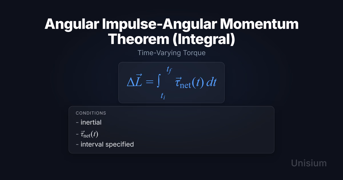
The Angular Impulse-Angular Momentum Theorem (Integral) states that the change in angular momentum of a system equals the time integral of the net torque acting on it: . This form applies when torque varies with time, requiring integration over the interval to find the cumulative rotational effect.
When net torque changes throughout a motion, such as a brake torque growing over time, a motor torque ramping up, or a measured torque-time graph, the constant-torque shortcut is not enough. The integral form accumulates torque over the interval to predict the change in angular momentum.
On this page: The Principle | Conditions | Misconceptions | EE Questions | Retrieval Practice | Worked Example | Solve a Problem | FAQ
The Principle
Statement
The change in angular momentum of a system between two instants equals the time integral of the net torque acting on the system over that interval. This is the general form that applies regardless of whether torque is constant or time-varying.
Mathematical Form
Where:
- = change in angular momentum ()
- = net torque as a function of time ()
- = initial and final times defining the interval ()
- The integral accumulates the rotational effect of torque over the entire interval
Alternative Forms
In different contexts, this appears as:
- Scalar (fixed axis): (for rotation about a single axis with signed torque)
- Constant torque special case: (when torque is constant over the interval; this is the simpler angular impulse form)
Conditions of Applicability
Condition: inertial; ; interval specified
Practical modeling notes
- Inertial reference frame: The theorem assumes measurements are made in a non-accelerating frame. In a rotating or accelerating frame, fictitious torques appear.
- Time-varying torque: This form is necessary when net torque changes during the motion (e.g., friction torque that depends on angular speed, or external forces that vary in time).
- Interval specified: You must integrate over a defined time interval . If the torque function is unknown or discontinuous, the integral may not be tractable analytically.
When It’s Not Directly Usable
- Non-inertial frames: In accelerating or rotating frames, you must account for fictitious torques (centrifugal, Coriolis) before applying the theorem.
- Unknown torque function: If isn’t known, you can’t compute the integral from first principles—you need a torque-time graph, measurements, or a model that links to or other state variables.
- No net torque: If for the entire interval, angular momentum is conserved and the integral is trivially zero.
Want the complete framework behind this guide? Read Masterful Learning.
Common Misconceptions
Misconception 1: “Integration is only needed for complicated torque functions”
The truth: The integral form is the general statement of the theorem. Even when torque is constant, the result comes from evaluating the integral with as a constant.
Why this matters: Recognizing the integral form as fundamental helps you understand that the constant-torque version is a special case, not a separate principle. When you encounter time-dependent torque, you know immediately to integrate.
Misconception 2: “You always need an explicit function to use this theorem”
The truth: You can evaluate the integral using graphical methods (area under a torque-time curve), average torque approximation, or by solving the differential equation when depends on or other state variables.
Why this matters: Students sometimes abandon the theorem when is not given explicitly, missing opportunities to use graphical reasoning, approximation methods, or kinematic constraints.
Misconception 3: “Angular momentum is always conserved if no external forces act”
The truth: For a system, total angular momentum is conserved when net external torque is zero. Internal forces (action-reaction pairs) redistribute angular momentum among parts but do not change the system total.
Why this matters: Confusing external forces with external torques leads to errors. A skater pulling in their arms has no external torque, so total angular momentum is conserved even though internal forces do work and change rotational kinetic energy.
Elaborative Encoding
Use these questions to build deep understanding. (See Elaborative Encoding for the full method.)
Within the Principle
- Why does the theorem involve an integral rather than just multiplying torque by elapsed time?
- What does the vector nature of and tell you about three-dimensional rotations?
For the Principle
- How do you decide whether torque is varying enough with time to require explicit integration, versus treating it as approximately constant?
- If you know the angular momentum at two instants but not the torque function, can you still use this theorem? What information would you extract?
Between Principles
- How does this integral form relate to the linear impulse-momentum theorem ?
Generate an Example
- Describe a realistic scenario where net torque varies smoothly with time (not a sudden impulse), requiring you to integrate to find the change in angular momentum.
Retrieval Practice
Answer from memory, then click to reveal and check. (See Retrieval Practice for the full method.)
State the angular impulse-momentum theorem (integral form) in words: _____The change in angular momentum of a system equals the time integral of the net torque acting on it over the interval.
Write the canonical equation for the integral form: _____
State the canonical condition: _____
Worked Example
Use this worked example to practice Self-Explanation.
Problem
A solid disk (moment of inertia ) rotates freely about a fixed axis. At , it spins at . A brake applies a time-varying frictional torque where . Find the angular velocity at .
Step 1: Verbal Decoding
Target: at
Given: , , ,
Constraints: fixed axis; friction torque opposes rotation; torque magnitude grows with time squared; no other torques
Step 2: Visual Decoding
Draw a disk rotating about a perpendicular axis through its center. Choose in the initial rotation direction. Mark opposite that direction.
(So and throughout the interval.)
Step 3: Physics Modeling
Step 4: Mathematical Procedures
Step 5: Reflection
- Units: ✓
- Magnitude: Final is much smaller than initial, consistent with braking torque that grows stronger over time.
- Limiting case: If (no torque), then , as expected.
Physics model with explanation
Principle: Angular impulse-momentum theorem (integral form) relates change in angular momentum to the time integral of net torque.
Conditions: Inertial frame; torque varies with time; interval specified.
Relevance: Since is time-varying (quadratic), the simple formula would be incorrect. We must integrate over the interval.
Description: The net torque is purely frictional and opposes rotation. It grows stronger as time progresses (quadratic dependence), so the disk slows down at an increasing rate.
Goal: Integrate the torque function to find the total angular impulse, then use the relation (for fixed ) to find the final angular velocity. The result shows the disk has slowed substantially but is still rotating.
Solve a Problem
Test your understanding with Problem Solving. Try it yourself before revealing the solution.
Click to show problem + solution
Problem
A thin rod (length , mass ) rotates about a perpendicular axis through one end. At , it is at rest. A time-varying torque where is applied for . Find the angular velocity at .
Step 1: Verbal Decoding
Target: at
Given: , , , ,
Constraints: axis through end; applied torque increases linearly with time; starts from rest
Step 2: Visual Decoding
Draw a rod pivoting about one end. Choose counterclockwise. Mark in that direction.
(So for all .)
Step 3: Physics Modeling
Step 4: Mathematical Procedures
Step 5: Reflection
- Units: ✓
- Magnitude: About revolutions per second is reasonable for a light rod with increasing torque over seconds.
- Limiting case: If (no torque), then , as expected.
Related Principles
- Classical Mechanics: The Complete Principle Map — see where this principle fits in the full subdomain.
| Principle | Relationship |
|---|---|
| Angular Impulse (Constant Torque) | Special case when is constant; then |
| Torque-Angular Momentum Form | Differential form: ; integrating this over time yields the impulse-momentum theorem |
| Angular Momentum Conservation | When net torque is zero, and angular momentum is conserved |
FAQ
When should I use the integral form instead of the constant-torque formula?
Use the integral form whenever net torque changes noticeably during the interval. If the problem statement gives or describes a varying force, you must integrate. If torque is approximately constant (or if the problem says “constant torque”), you can simplify to .
Can I evaluate the integral graphically if I don’t have an explicit function?
Yes. If you have a graph of torque versus time, the area under the curve from to gives . This is often easier than trying to fit an algebraic function to experimental data.
Does this theorem apply to multi-body systems, like a system of connected rigid bodies?
Yes, as long as you sum the torques from all external sources acting on the entire system about a common axis or center of mass. Internal torques (action-reaction pairs) cancel by Newton’s third law. The theorem then gives the change in total angular momentum of the system.
What if moment of inertia changes during the motion (e.g., a spinning skater pulling in their arms)?
The theorem still holds as long as you correctly account for external torques. If there is no external torque, (angular momentum is conserved) even though and individually change. When changing , use at each instant.
Is there an equivalent “power” or “work” version of this theorem for rotation?
Yes. The rotational work-energy theorem relates change in rotational kinetic energy to the work done by torques. The impulse-momentum form focuses on momentum changes over time, while work-energy focuses on energy changes over angular displacement. Both are correct but answer different questions.
How do I handle three-dimensional rotation where and are not parallel?
In 3D, is a vector equation, and can change direction even if its magnitude stays constant (precession). The integral form still holds as a vector equation. You integrate each component separately in a chosen coordinate system.
Can I use this theorem in a non-inertial reference frame?
You can, but you must add fictitious torques (due to the frame’s acceleration or rotation) to . It is usually simpler to work in an inertial frame and transform results afterward if needed.
Related Guides
- Five-Step Problem-Solving Strategy — Systematic approach to mechanics problems
- Rotational Kinetic Energy — Energy-based perspective on rotation
- Angular Impulse (Constant Torque) — Simpler form when torque is constant
How This Fits in Unisium
The Unisium Study System helps you master the angular impulse-momentum theorem (integral form) through elaborative encoding, retrieval practice, self-explanation, and problem solving. Our platform tracks your fluency with time-varying torque problems, generates targeted practice, and connects this principle to prerequisite concepts (like rotational kinematics) and advanced applications (like conservation laws in complex systems).
Ready to deepen your understanding? Start learning with Unisium or explore our research-backed approach in Masterful Learning.

Masterful Learning
The study system for physics, math, & programming that works: retrieval, connection, explanation, problem solving, and more.
Ready to apply this strategy?
Join Unisium and start implementing these evidence-based learning techniques.
Start Learning with Unisium Read More GuidesWant the complete framework? This guide is from Masterful Learning.
Learn about the book →