Velocity Change - Integral Relation: Find Velocity from Acceleration
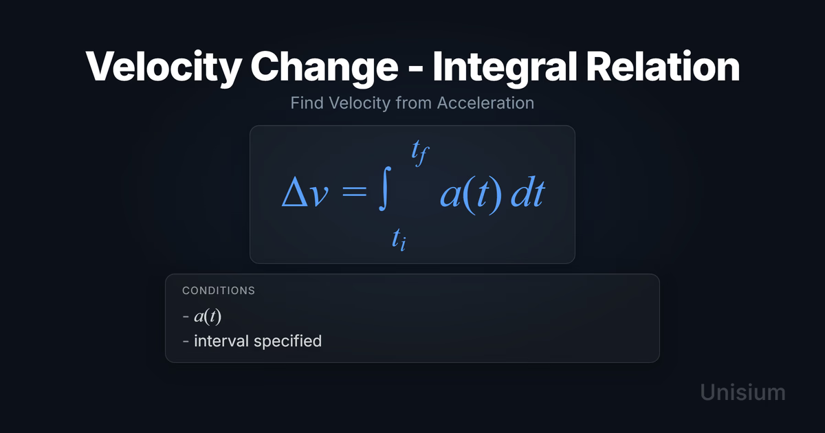
The velocity integral relation says that the change in velocity equals the time integral of acceleration over a specified interval: . Use it when acceleration is known as a function of time, especially when constant-acceleration formulas do not apply.
This relation is the continuous analog of summing acceleration over discrete time steps. It’s essential when acceleration varies with time—common in non-uniform motion, rocket propulsion, or any situation where forces change continuously. Unlike kinematic equations that assume constant acceleration, the integral form handles arbitrary acceleration profiles.
On this page: The Principle | Conditions | Misconceptions | EE Questions | Retrieval Practice | Worked Example | Solve a Problem | FAQ
The Principle
Statement
The velocity change of an object equals the time integral of its acceleration. When acceleration varies with time, you must integrate over the time interval to find the total velocity change. This connects velocity to acceleration through calculus, expressing the fundamental idea that acceleration is the instantaneous rate of velocity change.
Mathematical Form
Where:
- = change in velocity (m/s)
- = acceleration as a function of time (m/s)
- = initial time (s)
- = final time (s)
- = infinitesimal time interval (s)
Alternative Forms
In different contexts, this appears as:
- Velocity function (with initial condition):
- Vector form: (for two- or three-dimensional motion)
Conditions of Applicability
Condition: ; interval specified
This means:
- You must know acceleration as a function of time:
- The time interval must be specified or determinable
Practical modeling notes
- If acceleration is constant, the integral simplifies to (the traditional kinematic equation)
- For velocity-dependent or position-dependent forces, you may need to convert to first by solving differential equations
- In vector problems, apply the integral component-wise: ,
When It Doesn’t Apply
This relation fails or must be modified when:
- Acceleration depends on velocity or position: If or , you cannot directly integrate with respect to time. Instead, use chain rule techniques: or solve the differential equation .
- Discontinuous acceleration: At moments of abrupt force changes (collisions, instantaneous impulses), use the impulse-momentum theorem instead: .
- Unknown time dependence: If you don’t know how acceleration varies with time, you need more information (force laws, kinematic constraints) to construct before integrating.
Want the complete framework behind this guide? Read Masterful Learning.
Common Misconceptions
Misconception 1: “Integration just means multiply by time”
The truth: Integration accumulates infinitesimal contributions. When acceleration varies, you cannot simply multiply by . The integral accounts for how changes across the interval, weighting each instant appropriately.
Why this matters: Using when acceleration is non-constant yields incorrect results. For example, if (linearly increasing), the correct result is , not .
Misconception 2: “You need the anti-derivative to use this”
The truth: The integral is a tool, not a memorization task. If you cannot find an analytical anti-derivative (e.g., is given as a table or graph), you can use numerical integration (trapezoidal rule, Simpson’s rule) or graphical area-under-curve methods.
Why this matters: Physics problems often present data graphically or numerically. Recognizing that equals the area under an -vs- curve lets you solve problems even when symbolic integration is intractable.
Misconception 3: “This only works in one dimension”
The truth: The principle holds in all dimensions. For vector motion, apply the integral component-wise: , , . Or compactly: .
Why this matters: Projectile motion with air resistance, orbital mechanics with time-varying thrust, and charged particle motion in electric fields all require vector integration. Ignoring the vector nature leads to incorrect trajectories.
Elaborative Encoding
Use these questions to build deep understanding. (See Elaborative Encoding for the full method.)
Within the Principle
- What does represent physically in the integral ? Why does multiplying acceleration by an infinitesimal time interval give an infinitesimal velocity change?
- If acceleration is measured in m/s and time in seconds, verify that has units of m/s (velocity change).
For the Principle
- How do you decide whether to integrate over time versus using the chain rule ? What does it depend on?
- If you’re given a graph of versus , how would you determine without algebra?
Between Principles
- How does the velocity integral relate to the impulse-momentum theorem? Both involve integrating a rate over time—what’s the difference in what they calculate?
Generate an Example
- Describe a real-world situation where acceleration increases linearly with time (constant jerk), and explain why the simple formula would fail.
Retrieval Practice
Answer from memory, then click to reveal and check. (See Retrieval Practice for the full method.)
State the principle in words: _____The change in velocity equals the time integral of acceleration over the specified interval.
Write the canonical equation: _____
State the canonical condition: _____
Worked Example
Use this worked example to practice Self-Explanation.
Problem
A rocket fires its engines such that its vertical acceleration increases linearly from at to at . The rocket starts from rest. What is the rocket’s velocity at ?
Step 1: Verbal Decoding
Target: (velocity at )
Given: , , , ,
Constraints: Acceleration varies linearly with time; rocket starts from rest; vertical motion
Step 2: Visual Decoding
Choose upward. Label at the start and upward. (So is positive.) Sketch an -vs- graph showing acceleration increasing linearly from to over 5 seconds—the area under this line represents .
Step 3: Physics Modeling
Step 4: Mathematical Procedures
Step 5: Reflection
- Units: Integrating m/s over seconds yields m/s, as expected for velocity.
- Magnitude: The average acceleration is over , giving —consistent with our result.
- Limiting case: If acceleration were constant at , we’d get . The increasing acceleration produces a larger final velocity.
Before moving on: self-explain the model
Try explaining Step 3 out loud (or in writing): why the integral form applies, what the linear function represents, and how the equations encode the continuously increasing acceleration.
Physics model with explanation (what “good” sounds like)
Principle: The velocity integral relation, because we’re finding velocity change from a time-varying acceleration.
Conditions: Acceleration is given as a linear function of time, , over the interval —satisfying the condition “a(t); interval specified.”
Relevance: The constant-acceleration kinematic equations don’t apply here. We must integrate to account for how acceleration increases continuously.
Description: The rocket’s thrust increases steadily, causing acceleration to ramp up from to . The linear relationship captures this. Integrating this function over 5 seconds accumulates the velocity change, which equals the area under the -vs- line (a trapezoid with average height and width ).
Goal: We’re solving for final velocity. Since the rocket starts from rest, . The integration yields , confirming that the increasing acceleration delivers more velocity change than a constant would.
Solve a Problem
Apply what you’ve learned with Problem Solving.
Problem
A car decelerates such that its acceleration is m/s (where is in seconds). At , the car’s velocity is . What is the car’s velocity at ?
Hint: Set up the integral and evaluate the anti-derivative.
Show Solution
Step 1: Verbal Decoding
Target: at
Given: , , ,
Constraints: Acceleration varies linearly with time; car is decelerating; one-dimensional motion
Step 2: Visual Decoding
Choose in the direction of initial motion. Label positive and positive but smaller. (So both velocities are positive, but is negative.) Sketch an -vs- graph showing acceleration starting at and increasing to —the negative area represents the velocity decrease.
Step 3: Physics Modeling
Step 4: Mathematical Procedures
Step 5: Reflection
- Units: Acceleration integrated over time yields velocity change in m/s, correct.
- Magnitude: The car loses over 4 seconds, averaging , which is reasonable given the acceleration ranges from to .
- Limiting case: If acceleration were constant at , . The weakening deceleration (as increases toward zero) means the car slows less than it would with constant deceleration.
Related Principles
- Classical Mechanics: The Complete Principle Map — see where this principle fits in the full subdomain.
| Principle | Relationship to Velocity Integral |
|---|---|
| Acceleration as Derivative | The inverse operation: defines , which the velocity integral undoes |
| Displacement Integral | Parallel form: (one kinematic level higher) |
| Impulse-Momentum Theorem | Analogous structure: integrates force over time to get momentum change, |
See Principle Structures for how to organize these relationships visually.
FAQ
What is the Velocity Change - Integral Relation?
It states that the change in an object’s velocity over a time interval equals the integral of its acceleration over that interval: . This connects velocity and acceleration through calculus when acceleration varies with time.
When does the Velocity Integral apply?
It applies when acceleration is known as a function of time, , and you have a specified time interval over which to integrate. If acceleration is constant, the integral simplifies to the familiar .
What’s the difference between the Velocity Integral and the constant-acceleration equations?
The constant-acceleration equations (e.g., ) are special cases assuming is constant. The velocity integral handles any time-dependent acceleration—constant, linear, exponential, or even tabulated data.
What are the most common mistakes with the Velocity Integral?
- Treating non-constant acceleration as constant and using
- Forgetting to evaluate the definite integral at the correct limits
- Confusing with or and trying to integrate directly with respect to time when acceleration depends on velocity or position
How do I know which form of the Velocity Integral to use?
Use the scalar form for one-dimensional motion. For two- or three-dimensional motion, use the vector form or apply the scalar integral component-wise.
Related Guides
- Principle Structures — Organize the velocity integral in the kinematic hierarchy
- Retrieval Practice — Make this principle instantly accessible
- Self-Explanation — Learn to explain worked examples step by step
- Problem Solving — Apply principles systematically to new problems
How This Fits in Unisium
Unisium helps students master the velocity integral through targeted elaboration (connecting it to derivatives, impulse, and area-under-curve reasoning), spaced retrieval practice (recalling the equation and conditions on demand), self-explanation of worked examples (verbalizing why integration is necessary), and structured problem solving (applying it to realistic, variable-acceleration scenarios).
Ready to master the Velocity Integral? Start practicing with Unisium or explore the full learning framework in Masterful Learning.

Masterful Learning
The study system for physics, math, & programming that works: retrieval, connection, explanation, problem solving, and more.
Ready to apply this strategy?
Join Unisium and start implementing these evidence-based learning techniques.
Start Learning with Unisium Read More GuidesWant the complete framework? This guide is from Masterful Learning.
Learn about the book →