Linear Model: Understanding Slope and Intercept

This guide sits inside the Algebra study map, where you can see the neighboring moves, models, and next-step guides that connect this principle to the rest of algebra.

On this page: The Principle | Conditions | Misconceptions | EE Questions | Retrieval Practice | Worked Example | Solve a Problem | FAQ

---

The Principle

Statement

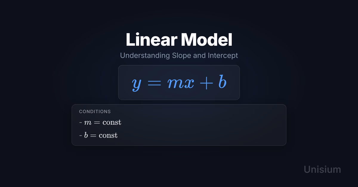
The Linear Model states that two quantities share a straight-line relationship described by $y = mx + b$, where $m$ (the slope) and $b$ (the $y$-intercept) are fixed constants. The slope measures the constant rate of change of $y$ with respect to $x$; the intercept gives the value of $y$ when $x = 0$. Any straight-line (affine) relationship fits this pattern; the Proportional Model ($y = kx$) is the special case $b = 0$.

Mathematical Form

$y = mx + b$

Where:

• $y$ = dependent variable (output)
• $x$ = independent variable (input)
• $m$ = slope; rate of change of $y$ per unit increase in $x$; units of $[y]/[x]$ (constant)
• $b$ = $y$-intercept; value of $y$ when $x = 0$; units of $[y]$ (constant)

Alternative Forms

In different contexts, the same principle appears as:

• Point-slope form: $y - y_1 = m(x - x_1)$ (useful when a point and slope are known)
• Slope from two points: $m = \dfrac{y_2 - y_1}{x_2 - x_1}$ (used to determine $m$ from two known data points)

---

Conditions of Applicability

Condition: $m=\mathrm{const}$; $b=\mathrm{const}$

The model holds when both the slope and the intercept are constant — they must not depend on $x$, $y$, or any other varying quantity.

Practical modeling notes

• In physical science, constant slope often follows from a constant rate of change (e.g., constant velocity, constant heating rate, constant drain rate).
• The Linear Model is technically an affine function (straight line, possibly offset). In everyday school algebra, “linear” includes a nonzero intercept; the Proportional Model $y = kx$ is the special case that passes through the origin ($b = 0$).
• When data appear roughly straight over a small range but curve globally, apply the model only within that range and state that restriction explicitly.

When It Doesn’t Apply

When $m$ or $b$ depends on the input, the relationship is nonlinear:

• Quadratic: $y = ax^2 + bx + c$ — the rate of change itself changes, so the graph curves.
• Exponential: $y = Ae^{kx}$ — slope grows or shrinks proportionally with $y$.

(When $b = 0$ the Linear Model reduces to the Proportional Model $y = kx$—that is a special case, not a failure of applicability.)

Want the complete framework behind this guide? Read Masterful Learning.

This model grows directly out of the Proportional Model when a nonzero intercept is added. Compare it with Exponential Model when the rate of change is no longer constant, and move next to Quadratic Model when the graph curves instead of staying straight.

---

Common Misconceptions

Misconception 1: The Linear Model and the Proportional Model are the same thing

The truth: The Proportional Model $y = kx$ is a special case of the Linear Model where $b = 0$. When $b \neq 0$, the line does not pass through the origin, and $y/x$ is not constant.

Why this matters: Temperature conversion $F = \tfrac{9}{5}C + 32$ is linear but not proportional. Treating it as proportional gives $F \approx 1.8 C$, which is wrong at every temperature except $C = 0$.

Misconception 2: The slope $m$ must be positive

The truth: The slope can be negative (line falls left-to-right), zero (horizontal line), or positive. A negative slope means $y$ decreases as $x$ increases.

Why this matters: Signing errors for declining quantities (draining tanks, cooling temperatures, deceleration) often come from an implicit assumption that slope is positive. Always read the direction of change from the problem before assigning a sign.

Misconception 3: The letters $x$, $y$, $m$, and $b$ must be used

The truth: The model is a structural pattern — output equals slope times input plus intercept — that can use any variable names. You will encounter $v = at + v_0$, $F = \tfrac{9}{5}C + 32$, and $C = -250t + 3000$ in different contexts, all built on the same relationship.

Why this matters: Students who memorize only $y = mx + b$ often fail to recognize the model in different notation. Focus on identifying slope and intercept regardless of the letters used.

---

Elaborative Encoding

Use these questions to build deep understanding of the Linear Model. (See Elaborative Encoding for the full strategy.)

Within the Principle

• In $y = mx + b$, what are the units of $m$ if $y$ is measured in meters and $x$ in seconds? What physical quantity does $m$ represent in that case?
• If $m$ is doubled while $b$ stays the same, how does the graph change? What if $b$ is doubled while $m$ stays the same?

For the Principle

• A quantity increases at a constant rate from a nonzero starting value. How do you identify which part of the problem gives you $m$ and which gives you $b$?
• How do you decide whether to use the Linear Model or the Proportional Model ($y = kx$)? What property of the data or scenario signals that $b \neq 0$?

Between Principles

• The Proportional Model ($y = kx$) is a special case of the Linear Model. What condition on $b$ produces the Proportional Model, and what changes about the graph when that condition is met?

Generate an Example

• Describe a real situation where a quantity changes at a constant rate but starts at a nonzero value. Write the equation, identify $m$ and $b$, and explain what each constant means in that context.

---

Retrieval Practice

Answer from memory, then click to reveal and check. (See Retrieval Practice for the full strategy.)

State the Linear Model in words: _____The output equals the slope times the input plus a constant intercept; both slope and intercept are fixed constants.

Write the canonical equation: _____$y = mx + b$

State the canonical condition: _____$m=\mathrm{const}; b=\mathrm{const}$

---

Worked Example

Use this worked example to practice Self-Explanation.

Problem

The boiling point of water is $212\,°\mathrm{F}$ at $100\,°\mathrm{C}$, and the freezing point is $32\,°\mathrm{F}$ at $0\,°\mathrm{C}$. Using these two data points, find the linear equation for Fahrenheit $F$ as a function of Celsius $C$. Then find the Celsius temperature corresponding to $77\,°\mathrm{F}$.

Step 1: Verbal Decoding

Target: (a) equation $F(C)$; (b) $C$ at $F = 77\,°\mathrm{F}$
Given: $C_1, F_1, C_2, F_2, F$
Constraints: linear relation; $m = \mathrm{const}$; $b = \mathrm{const}$

Step 2: Visual Decoding

Draw 2D axes: choose $+C$ to the right and $+F$ upward. Plot the two given points and draw the straight line through them. (So $\Delta C > 0$ and $\Delta F > 0$ between the points, confirming $m > 0$.)

Step 3: Mathematical Modeling

1. $F = m\,C + b$

Step 4: Mathematical Procedures

1. $m = \frac{F_2 - F_1}{C_2 - C_1}$
2. $m = \frac{(212 - 32)\,°\mathrm{F}}{(100 - 0)\,°\mathrm{C}}$
3. $m = \frac{180}{100}\,\frac{°\mathrm{F}}{°\mathrm{C}}$
4. $m = \frac{9}{5}\,\frac{°\mathrm{F}}{°\mathrm{C}}$
5. $b = F_1 - m\,C_1$
6. $b = 32\,°\mathrm{F} - \frac{9}{5}\,\frac{°\mathrm{F}}{°\mathrm{C}}\,(0\,°\mathrm{C})$
7. $b = 32\,°\mathrm{F}$
8. $F(C) = \frac{9}{5}\,C + 32$
9. $C = \frac{F - b}{m}$
10. $C = \frac{(77 - 32)\,°\mathrm{F}}{\tfrac{9}{5}\,°\mathrm{F}/°\mathrm{C}}$
11. $C = \frac{45}{9/5}\,°\mathrm{C}$
12. $\underline{F(C) = \tfrac{9}{5}\,C + 32,\quad C = 25\,°\mathrm{C}}$

Step 5: Reflection

• Units: slope $m$ has units $°\mathrm{F}/°\mathrm{C}$ and intercept $b$ has units $°\mathrm{F}$, so every term in $F(C)$ is in $°\mathrm{F}$.
• Verification: at $C = 100\,°\mathrm{C}$: $F = \tfrac{9}{5}(100) + 32 = 212\,°\mathrm{F}$ ✓ — matches the known boiling point used to build the model.
• Plausibility: $25\,°\mathrm{C}$ for $77\,°\mathrm{F}$ is a warm spring day — realistic.

---

Before moving on: self-explain the model

Try explaining Step 3 out loud: why the Linear Model applies, what the two given points tell you, and how Steps 4–5 uniquely determine the equation.

Mathematical model with explanation

Principle: Linear Model — $F(C) = \tfrac{9}{5}C + 32$ is a straight-line (affine) function with constant slope and intercept.

Conditions: The relationship between Fahrenheit and Celsius is exactly linear by construction of the temperature scales, so both $m$ and $b$ are constants. The condition $m=\mathrm{const}$; $b=\mathrm{const}$ is satisfied.

Relevance: Two distinct points uniquely determine a line. Knowing the freezing and boiling points supplies exactly that information, making this a direct application of the two-point slope formula.

Description: We computed $m$ using the slope formula from the two known data points, then read $b$ directly from the point at $C = 0$ (where the $mC$ term vanishes). Once the equation is established, finding $C$ from $F$ is a one-step algebraic solve.

Goal: Express $F$ as a function of $C$, then invert the equation to recover the Celsius value corresponding to $F = 77$.

---

Solve a Problem

Apply what you have learned with Problem Solving.

Problem

A water tank contains $3{,}000$ liters when monitoring begins at $t = 0$. Water drains at a constant rate of $250$ liters per hour.

(a) Write the linear equation for volume $V$ (in liters) remaining after $t$ hours.
(b) How many hours until the tank is empty?

Hint (if needed): A constant drain rate produces a constant slope. Which direction should the slope point, and what is the $y$-intercept of $V(t)$?

Show Solution

Step 1: Verbal Decoding

Target: (a) equation $V(t)$; (b) $t^*$ when $V = 0$
Given: $V_0,\, r$
Constraints: constant drain rate; volume decreases linearly

Step 2: Visual Decoding

Draw 2D axes: choose $+t$ to the right and $+V$ upward with $t = 0$ at the start. Draw a line from a positive $V$-intercept sloping downward. (So $\Delta V < 0$ as $t$ increases, confirming $m < 0$.)

Step 3: Mathematical Modeling

1. $V(t) = m\,t + V_0$

Step 4: Mathematical Procedures

1. $V(t) = -r\,t + V_0$
2. $V(t) = -250\,t + 3000$
3. $0 = -250\,t^* + 3000$
4. $250\,t^* = 3000$
5. $t^* = \frac{3000\,\mathrm{L}}{250\,\mathrm{L/hr}}$
6. $\underline{V(t) = -250\,t + 3000,\quad t^* = 12\,\mathrm{hr}}$

Step 5: Reflection

• Units: slope $m$ has units $\mathrm{L/hr}$ and $V_0$ has units $\mathrm{L}$, so $V(t)$ is in liters and $t^* = V_0/r$ has units $\mathrm{L}/(\mathrm{L/hr}) = \mathrm{hr}$.
• Verification: $V(12) = -250(12) + 3000 = 0$ ✓ — the tank is exactly empty at $t^* = 12\,\mathrm{hr}$.
• Parameter dependence: doubling the drain rate to $500\,\mathrm{L/hr}$ halves the empty time to $6\,\mathrm{hr}$ — $t^*$ is inversely proportional to $r$.

---

Related Principles

Principle	Relationship to the Linear Model
Proportional Model	Special case $b = 0$: the line passes through the origin and the ratio $y/x$ is constant.
Slope from Two Points	The formula $m = (y_2 - y_1)/(x_2 - x_1)$ is the standard procedure for computing the slope from data; no separate principle key yet.
Quadratic Model	The next-degree generalization; the slope is no longer constant (it depends on $x$), so $m = \mathrm{const}$ fails. No separate principle key yet.

Only linked items are registered Unisium principles; unlinked rows are conceptual neighbors pending a principle key.

---

FAQ

What is the Linear Model?

The Linear Model is the equation $y = mx + b$, where slope $m$ and intercept $b$ are constants. It represents any relationship that forms a straight line on a graph. The slope gives the constant rate of change; the intercept gives the value of $y$ at $x = 0$.

When does the Linear Model apply?

It applies when two quantities are related by a constant rate of change and a fixed starting value — both $m$ and $b$ must be constants, independent of $x$ and $y$. You can verify this by checking whether a graph of the data is straight, or whether the problem explicitly states a constant rate from some initial value.

What is the difference between the Linear Model and the Proportional Model?

The Proportional Model $y = kx$ requires the line to pass through the origin ($b = 0$), so the ratio $y/x$ is constant. The Linear Model allows any intercept. If a problem has a nonzero starting value and a constant rate, use the Linear Model.

What does the slope $m$ represent?

The slope is the rate of change of $y$ per unit increase in $x$. Its units are always (units of $y$) divided by (units of $x$). A positive slope means $y$ increases with $x$; a negative slope means $y$ decreases.

What are the most common mistakes with the Linear Model?

The three most frequent errors are: (1) confusing linear with proportional by neglecting the intercept $b$; (2) assigning the wrong sign to slope when the quantity is decreasing; and (3) substituting numerical values before establishing a symbolic equation, which hides structure and leads to arithmetic errors.

How do I find the equation from a graph or two points?

Compute slope from two points using $m = (y_2 - y_1)/(x_2 - x_1)$, then substitute one point into $y = mx + b$ to solve for $b$. If one of the points is the $y$-intercept $(0, b_0)$, read $b$ directly. The result is the unique line through those two points.

---

Related Guides

• Self-Explanation — Use the worked example above to practice this strategy on a real algebraic model
• Retrieval Practice — Make the equation and condition instantly accessible from memory
• Elaborative Encoding — Build the deep understanding needed to recognize and apply the model flexibly
• Problem Solving — Apply the Five-Step Strategy systematically to problems involving linear relationships

---

How This Fits in Unisium

Unisium tracks the Linear Model as a foundational algebra principle that appears across math, physics, chemistry, and economics. In practice, the app presents elaborative encoding questions that probe what $m$ and $b$ mean in a specific context, schedules retrieval cloze prompts so you recall the equation and condition under time pressure, and provides structured problem-solving exercises with immediate step-level feedback. Because the model recurs in dozens of downstream topics, building reliable fluency here compounds across your entire curriculum.

Ready to master the Linear Model? Start practicing with Unisium or explore the full learning framework in Masterful Learning.

Masterful Learning

The study system for physics, math, & programming that works: retrieval, connection, explanation, problem solving, and more.

Read the book (opens in new tab) ISBN 979-8-2652-9642-9