Exponential Model: Equal Multiplier per Unit Input

This guide sits inside the Algebra study map, where you can see the neighboring moves, models, and next-step guides that connect this principle to the rest of algebra.

On this page: The Principle · Conditions · Misconceptions · EE Questions · Retrieval Practice · Worked Example · Solve a Problem · FAQ

---

The Principle

Statement

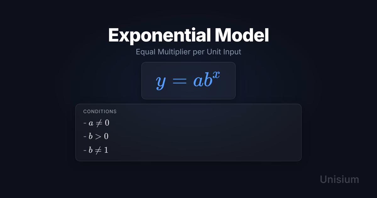
The Exponential Model states that the output $y$ equals a nonzero initial value $a$ multiplied by a positive base $b \neq 1$ raised to the power $x$. Each unit increase in $x$ multiplies the previous output by $b$—the defining feature that distinguishes exponential change from linear (constant additive change) and quadratic (constant second-difference change).

Mathematical Form

$y = ab^x$

Where:

• $y$ = the output quantity
• $a$ = initial value; the output when $x = 0$ (must be nonzero)
• $b$ = base; the constant multiplier applied per unit increase in $x$ ($b > 0$, $b \neq 1$)
• $x$ = the input variable (often representing time, steps, or equal-width intervals)

Alternative Forms

In applied contexts this model is often rewritten to make the rate explicit:

• Rate form: $y = a(1+r)^x$ — where $r$ is the per-unit growth rate ($r > -1$, $r \neq 0$); the base is $b = 1+r$

---

Conditions of Applicability

Condition: $a \neq 0$; $b>0$; $b\neq 1$

The deeper applicability test is structural: the situation must produce a constant ratio between consecutive outputs at equal input steps. Verify this before fitting the model. The parameter restrictions below then ensure the equation is non-trivial and well-defined over real inputs.

Practical modeling notes

• $a \neq 0$: if $a = 0$ the output is zero for every $x$, which is trivially constant and carries no exponential information.
• $b > 0$: a negative base produces undefined real outputs for fractional exponents and oscillates in sign, neither of which matches the constant-ratio growth or decay behavior the model describes.
• $b \neq 1$: the base $b = 1$ gives $y = a \cdot 1^x = a$ for all $x$—a horizontal line, not an exponential function.

When It Doesn’t Apply

• Constant output: If $b = 1$, the model degenerates to the constant function $y = a$. A Linear Model or direct inspection is appropriate instead.
• Negative base: When $b < 0$, $b^x$ is undefined for most real $x$ values. A separate convention (complex exponentiation) is required; the real exponential model does not apply.
• Variable rate: If the multiplicative factor changes with $x$, the relationship is no longer exponential. A different model type is needed.

Want the complete framework behind this guide? Read Masterful Learning.

Compare this with Linear Model when deciding whether a constant difference or a constant ratio drives the change. A useful next contrast is Quadratic Model when the data curve but do not grow multiplicatively.

---

Common Misconceptions

Misconception 1: “When $x = 0$, the output is zero”

The truth: At $x = 0$, $b^0 = 1$, so $y = a \cdot 1 = a$. The output equals the initial value $a$, not zero. That is why $a$ is called the initial value and why this guide defines the non-trivial exponential model with the condition $a \neq 0$.

Why this matters: Misreading the $y$-intercept as zero leads to an incorrect model. Students who confuse $y = ab^x$ with a function that starts at the origin build wrong equations and make systematic errors in every subsequent step.

Misconception 2: “Any base works, including $b = 1$”

The truth: $b = 1$ produces the constant function $y = a$, not an exponential. The defining property of an exponential model is that the output changes by a constant factor each step. With $b = 1$ that factor is exactly 1, meaning no change at all.

Why this matters: The condition $b \neq 1$ is part of the principle definition, not an optional restriction. Accepting $b = 1$ in a model silently removes all exponential behavior while the equation still looks correct.

Misconception 3: “A negative base such as $b = -2$ is fine as long as its magnitude exceeds 1”

The truth: The condition requires $b > 0$. When $b < 0$, expressions like $(-2)^{1/2}$ have no real value, so the model is undefined for most real inputs. The function also alternates in sign as $x$ steps through integers, which does not correspond to real-world growth or decay.

Why this matters: Students who accept a negative base create a function that is undefined over most of the real line. Checking $b > 0$ before writing the model prevents this undefined behavior.

---

Elaborative Encoding

Use these questions to build deep understanding. (See Elaborative Encoding for the full method.)

Within the Principle

• In $y = ab^x$, what numeric value does the function output when $x = 0$? Trace through the exponent rule $b^0 = 1$ and state what this says about the role of $a$.
• If $b = 3$ and $a = 4$, by what factor does $y$ change when $x$ increases from 2 to 3? From 5 to 6? What does the fact that these factors are equal tell you about the model?

For the Principle

• A data table shows values at equal $x$-intervals. What calculation would you perform on consecutive output values to decide whether an exponential model is appropriate, and what result would confirm it?
• Give an example of a situation where you would write $b = 1 + r$ with $0 < r < 1$ versus $b = 1 + r$ with $r < 0$. What real-world context distinguishes growth ($r > 0$) from decay ($r < 0$)?

Between Principles

• Compare $y = ab^x$ with the Linear Model $y = mx + c$. For both, state what property of consecutive outputs (differences vs. ratios) is constant, and explain why this structural difference makes the two models suited to different situations.

Generate an Example

• Write a scenario where the exponential model applies, then deliberately violate one condition ($a \neq 0$, $b > 0$, or $b \neq 1$). Describe what changes in the behavior of the function when that condition fails.

---

Retrieval Practice

Answer from memory, then click to reveal and check. (See Retrieval Practice for the full method.)

State the principle in words: _____The Exponential Model states that y equals a nonzero initial value a multiplied by a positive base b (not equal to 1) raised to the power x. Each unit increase in x multiplies the output by the same constant factor b.

Write the canonical equation: _____$y = ab^x$

State the canonical condition: _____$a \neq 0; b>0; b\neq 1$

---

Worked Example

Use this worked example to practice Self-Explanation.

Problem

A bacterial culture starts with 300 cells. The count triples every hour. Write the exponential model for the number of cells $y$ after $x$ hours, then find the count after 4 hours.

Step 1: Verbal Decoding

Target: model for $y$; $y$ at $x = 4$
Given: $a$, $b$, $x$
Constraints: initial value known; equal 1-hour intervals; constant multiplicative change

Step 2: Visual Decoding

Draw axes with $x$ = hours and $y$ = cell count. Mark $(0, 300)$. Sketch an increasing curve that rises steeply to the right.

Step 3: Mathematical Modeling

1. $y = 300 \cdot 3^x$

Step 4: Mathematical Procedures

1. $y = 300 \cdot 3^4$
2. $y = 300 \cdot 81$
3. $\underline{y = 24{,}300 \text{ cells}}$

Step 5: Reflection

• Verification: At $x = 0$, $y = 300 \cdot 3^0 = 300 \cdot 1 = 300$ ✓ — the initial value is recovered.
• Domain check: $a = 300 \neq 0$; $b = 3 > 0$; $b = 3 \neq 1$ — all three conditions satisfied.
• Connection to concept: Since $b = 3$, the output triples each time $x$ increases by 1, which is exactly the constant-ratio definition of exponential growth.

---

Before moving on: self-explain the model

Explain Step 3 in your own words: why does “triples every hour” translate directly to $b = 3$? How does the exponent $x$ encode the repeated multiplication by 3?

Mathematical model with explanation

Principle: Exponential Model, instantiated as $y = 300 \cdot 3^x$ with $a = 300$ and $b = 3$.

Conditions: $a = 300 \neq 0$; $b = 3 > 0$; $b = 3 \neq 1$ — all satisfied ✓.

Relevance: The problem states a constant tripling factor per hour, which matches the defining property of $y = ab^x$: the output is multiplied by $b$ for each unit increase in $x$.

Description: The initial count $a = 300$ is multiplied by $b = 3$ once per hour. After $x$ hours, the accumulated multiplier is $3^x$, giving the total cell count as $300 \cdot 3^x$.

Goal: Substitute $x = 4$ into the model, apply the exponent, and multiply to read off the population at that hour.

---

Solve a Problem

Apply what you’ve learned with Problem Solving.

Problem

An investment of 2,000 dollars grows at a fixed rate of 5% per year. Write the exponential model for its value $V$ after $t$ years, then find $V$ when $t = 6$.

Hint (if needed): A 5% annual increase means each year’s value is multiplied by $1 + 0.05$. Express the growth factor as a decimal, then use it as $b$.

Show Solution

Step 1: Verbal Decoding

Target: model for $V$; $V$ at $t = 6$
Given: $a$, $b$, $t$
Constraints: initial value known; equal 1-year intervals; constant multiplicative change

Step 2: Visual Decoding

Draw axes with $t$ = years and $V$ = value in dollars. Mark $(0, 2000)$. Sketch an increasing curve that rises gradually to the right.

Step 3: Mathematical Modeling

1. $V = 2000 \cdot (1.05)^t$

Step 4: Mathematical Procedures

1. $V = 2{,}000 \cdot (1.05)^6$
2. $V \approx 2{,}000 \cdot 1.34010\ldots$
3. $\underline{V \approx 2{,}680.19 \text{ dollars}}$

Step 5: Reflection

• Verification: At $t = 0$, $V = 2000 \cdot (1.05)^0 = 2000 \cdot 1 = 2000$ ✓ — matches the initial investment.
• Connection to concept: The base $1.05 > 1$ produces growth; each year the previous value is multiplied by the same factor, confirming constant-ratio behavior.
• Domain check: $a = 2000 \neq 0$; $b = 1.05 > 0$; $b = 1.05 \neq 1$ — all conditions satisfied.

---

Related Principles

Principle	Relationship to Exponential Model
Linear Model	Linear change adds a constant to the output per unit input; exponential change multiplies. Constant differences vs. constant ratios.
Quadratic Model	Quadratic relationships are identified by constant second differences, while exponential relationships are identified by constant ratios. Both can curve, but they encode different structures.
Negative Exponent Rule	Exponential decay ($0 < b < 1$) can be rewritten using the negative exponent rule: a base less than 1 is the reciprocal of a base greater than 1, connecting decay and growth forms of the same expression.

See Principle Structures for how to organize these relationships visually.

---

FAQ

What is the Exponential Model?

The Exponential Model is $y = ab^x$, where $a$ is the initial value, $b$ is a positive constant base not equal to 1, and $x$ is the input. The defining feature is that each unit increase in $x$ multiplies the output by the same factor $b$—constant ratio growth or decay.

When does the Exponential Model apply?

It applies when consecutive output values at equal input intervals have a constant ratio. Verify this by dividing successive outputs: if the quotient is constant, an exponential model fits. The conditions $a \neq 0$, $b > 0$, and $b \neq 1$ must all hold for the model to be non-trivial.

What is the difference between exponential growth and exponential decay?

Both use $y = ab^x$ with the same conditions. When $b > 1$, each step multiplies by a factor greater than 1, so output increases — this is growth. When $0 < b < 1$, each step multiplies by a fraction less than 1, so output decreases — this is decay. The sign of $a$ determines whether the curve lies above or below the $x$-axis.

What happens if the base $b$ equals 1?

The model collapses to the constant function $y = a \cdot 1^x = a$ for all $x$. There is no growth or decay — the output never changes. This is why $b \neq 1$ is required: the condition defines a meaningful exponential relationship.

How is the Exponential Model different from the Linear Model?

A Linear Model has a constant additive change per unit input (constant differences). The Exponential Model has a constant multiplicative change per unit input (constant ratios). This structural difference — not just the shape of the curve — determines which model is appropriate for a given situation.

---

Related Guides

• Principle Structures — Organize the Exponential Model in the algebra principle hierarchy
• Self-Explanation — Practice explaining each step of the worked example above
• Retrieval Practice — Make $y = ab^x$ and its conditions instantly accessible
• Problem Solving — Apply the Five-Step Strategy to exponential modeling problems systematically

---

How This Fits in Unisium

Unisium pairs the Exponential Model—like every principle in the algebra sequence—with elaborative-encoding questions, retrieval cloze prompts, and graded problem sets so you develop both rapid recall and flexible application. Working through the constant-ratio logic in EE questions, retrieving the equation and conditions from memory, then applying the Five-Step Strategy in worked and solo problems shortens the path from first exposure to reliable use under exam pressure.

Ready to master the Exponential Model? Start practicing with Unisium or explore the full learning framework in Masterful Learning.

Masterful Learning

The study system for physics, math, & programming that works: retrieval, connection, explanation, problem solving, and more.

Read the book (opens in new tab) ISBN 979-8-2652-9642-9