Kinematics 4: Displacement from Average Velocity

On this page: The Principle · Conditions · Misconceptions · EE Questions · Retrieval Practice · Worked Example · Solve a Problem · FAQ

This principle is one of four standard kinematics equations for constant acceleration motion. It’s particularly useful when you know velocities and time but not acceleration directly, making it a complement to the other kinematic relationships.

---

The Principle

Statement

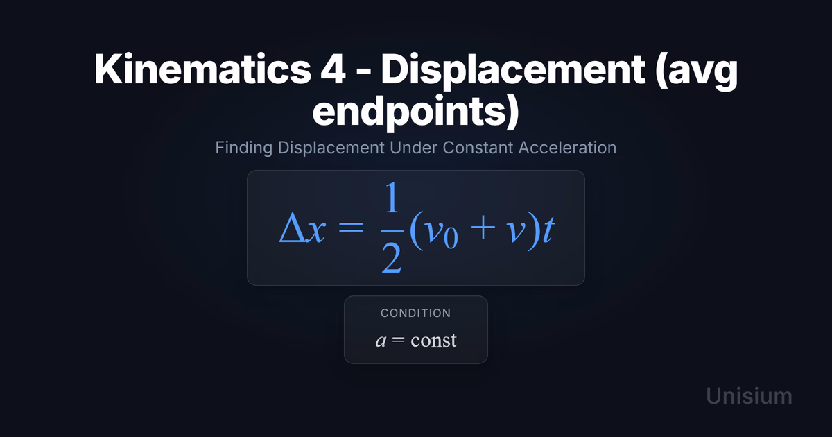
For motion with constant acceleration, the displacement equals the average of the initial and final velocities multiplied by the time interval. This follows from the fact that velocity changes linearly with time when acceleration is constant, so the arithmetic mean of the endpoint velocities gives the average velocity over the interval.

Mathematical Form

$\Delta x = \frac{1}{2}(v_0 + v)t$

Where:

• $\Delta x$ = displacement (change in position), in meters (m)
• $v_0$ = initial velocity, in meters per second (m/s)
• $v$ = final velocity, in meters per second (m/s)
• $t$ = time interval, in seconds (s)

Alternative Forms

In different contexts, this appears as:

• Explicit average velocity: $\bar{v} = \frac{v_0 + v}{2}$, then $\Delta x = \bar{v} t$
• Expanded form: $\Delta x = \bar{v} t$ where $\bar{v}$ is the average velocity

---

Conditions of Applicability

Condition: $a=\mathrm{const}$ The equation assumes acceleration is constant throughout the time interval. This is the same condition that applies to all four standard kinematics equations.

Practical modeling notes

• Motion under constant gravitational acceleration near Earth’s surface satisfies this condition (neglecting air resistance)
• Motion with zero net force (constant velocity) is a special case with $a = 0$
• For problems involving changing acceleration, you must break the motion into segments where acceleration is approximately constant
• For rotational problems, use the angular analog $\Delta \theta = \frac{1}{2}(\omega_0 + \omega)t$ under constant $\alpha$

When It Doesn’t Apply

• Variable acceleration: When forces change with position or time (e.g., spring force, air resistance proportional to velocity), you must use calculus-based methods or other kinematic principles

Want the complete framework behind this guide? Read Masterful Learning.

---

Common Misconceptions

Misconception 1: The average velocity is always halfway between initial and final positions

The truth: Average velocity is displacement divided by time, which for constant acceleration equals the arithmetic mean of initial and final velocities, not positions.

Why this matters: Confusing average velocity with midpoint position leads to incorrect calculations, especially when initial position is not zero.

Misconception 2: This equation works for any motion as long as you know the velocities

The truth: The equation requires constant acceleration; for variable acceleration, the average velocity is not simply $\frac{v_0 + v}{2}$.

Why this matters: Applying this formula when acceleration varies (like in circular motion at changing speed) produces wrong answers.

Misconception 3: You need to know acceleration to use this equation

The truth: This equation bypasses acceleration entirely, requiring only velocities and time.

Why this matters: Recognizing when to use Kinematics 4 instead of Kinematics 1 or 2 (which explicitly involve acceleration) saves steps and reduces error propagation.

---

Elaborative Encoding

Use these questions to build deep understanding. (See Elaborative Encoding for the full method.)

Within the Principle

• Why does the arithmetic mean of $v_0$ and $v$ give the average velocity when acceleration is constant?
• What are the units of each term, and how do they combine to give displacement in meters?

For the Principle

• How do you decide whether to use Kinematics 4 versus Kinematics 1 ($v = v_0 + at$) in a problem?
• When you’re given initial velocity, final velocity, and displacement, why is Kinematics 4 not immediately useful?

Between Principles

• How is Kinematics 4 related to Kinematics 3 ($v^2 = v_0^2 + 2a\Delta x$), and when would you use one versus the other?

Generate an Example

• Describe a situation where you know $v_0$, $v$, and $\Delta x$, but Kinematics 4 cannot directly give you the answer you need.

---

Retrieval Practice

Answer from memory, then click to reveal and check. (See Retrieval Practice for the full method.)

State the principle in words: _____For constant acceleration, displacement equals the average of initial and final velocities multiplied by the time interval.

Write the canonical equation: _____$\Delta x = \frac{1}{2}(v_0 + v)t$

State the canonical condition: _____$a=\mathrm{const}$

---

Worked Example

Use this worked example to practice Self-Explanation.

Problem

A car accelerates uniformly from rest to 25 m/s in 8.0 s. How far does it travel during this time?

Step 1: Verbal Decoding

Target: $\Delta x$
Given: $v_0$, $v$, $t$
Constraints: Uniformly accelerating motion (constant acceleration), starts from rest

Step 2: Visual Decoding

Draw a horizontal axis representing the car’s path. Choose $+x$ in the direction of motion. Label the initial point (at rest) and final point (moving at 25 m/s). The car moves in the $+x$ direction throughout. (So $v_0 = 0$ and $v$ is positive.)

Step 3: Physics Modeling

1. $\Delta x = \frac{1}{2}(v_0 + v)t$

Step 4: Mathematical Procedures

1. $\Delta x = \frac{1}{2}(0\,\mathrm{m/s} + 25\,\mathrm{m/s})(8.0\,\mathrm{s})$
2. $\Delta x = \frac{1}{2}(25\,\mathrm{m/s})(8.0\,\mathrm{s})$
3. $\Delta x = 100\,\mathrm{m}$
4. $\underline{\Delta x = 1.0 \times 10^2\,\mathrm{m}}$

Step 5: Reflection

• Units: $(\mathrm{m/s})(\mathrm{s}) = \mathrm{m}$, as expected for displacement.
• Magnitude: 100 m is plausible for a car accelerating to highway speed over 8 seconds.
• Limiting case: If $v = v_0$ (constant velocity), $\Delta x = v_0 t$, which matches uniform motion.

---

Before moving on: self-explain the model

Try explaining Step 3 out loud (or in writing): why the chosen principle applies, what the diagram implies, and how the equations encode the situation.

Physics model with explanation (what “good” sounds like)

Principle: Kinematics 4 relates displacement to the average of initial and final velocities under constant acceleration.

Conditions: The problem states “uniformly accelerating,” which means constant acceleration, satisfying the condition $a = \mathrm{constant}$.

Relevance: We’re given $v_0$, $v$, and $t$, and asked for $\Delta x$. Kinematics 4 directly connects these four quantities without needing to find acceleration first.

Description: The car starts from rest ($v_0 = 0$) and reaches 25 m/s in 8.0 s. Because acceleration is constant, the average velocity is simply the arithmetic mean of initial and final velocities. Multiplying this average velocity by time gives the displacement.

Goal: We multiply the average velocity by the time interval to find how far the car travels during its acceleration phase.

---

Solve a Problem

Apply what you’ve learned with Problem Solving.

Problem

A cyclist slows uniformly from 12 m/s to 4.0 m/s over 6.0 s. What distance does the cyclist travel during this deceleration?

Hint: Even though the cyclist is slowing down, the average velocity formula still applies under constant acceleration.

Show Solution

Step 1: Verbal Decoding

Target: $\Delta x$
Given: $v_0$, $v$, $t$
Constraints: Uniform deceleration (constant acceleration), moving in one direction

Step 2: Visual Decoding

Draw a horizontal axis representing the cyclist’s path. Choose $+x$ in the initial direction of motion. Label the initial velocity (12 m/s) and final velocity (4.0 m/s), both positive. The cyclist continues forward but slows down. (So $v_0$ and $v$ are both positive.)

Step 3: Physics Modeling

1. $\Delta x = \frac{1}{2}(v_0 + v)t$

Step 4: Mathematical Procedures

1. $\Delta x = \frac{1}{2}(12\,\mathrm{m/s} + 4.0\,\mathrm{m/s})(6.0\,\mathrm{s})$
2. $\Delta x = \frac{1}{2}(16\,\mathrm{m/s})(6.0\,\mathrm{s})$
3. $\Delta x = 48\,\mathrm{m}$
4. $\underline{\Delta x = 48\,\mathrm{m}}$

Step 5: Reflection

• Units: $(\mathrm{m/s})(\mathrm{s}) = \mathrm{m}$, correct for displacement.
• Magnitude: 48 m for 6 seconds of slowing from 12 to 4 m/s is reasonable—average velocity is 8 m/s, so $8 \times 6 = 48$ m checks out.
• Limiting case: If the cyclist maintained 12 m/s for 6 s, displacement would be 72 m; if maintained 4 m/s, it would be 24 m. Our answer of 48 m is between these bounds, as expected.

---

Related Principles

• Classical Mechanics: The Complete Principle Map — see where this principle fits in the full subdomain.

Principle	Relationship to Kinematics 4
Kinematics 1	Gives $v$ from $v_0$, $a$, $t$; combine with K4 when $a$ is needed
Kinematics 2	Directly gives $\Delta x$ from $v_0$, $a$, $t$ without needing final velocity
Kinematics 3	Relates $v^2$ to $\Delta x$ without time; use when time is unknown

See Principle Structures for how to organize these relationships visually.

---

FAQ

What is Kinematics 4 - Average Velocity?

Kinematics 4 is the equation $\Delta x = \frac{1}{2}(v_0 + v)t$, which calculates displacement from the average of initial and final velocities multiplied by time. It applies to motion with constant acceleration.

When does Kinematics 4 apply?

It applies when acceleration is constant ($a = \mathrm{constant}$) and you know or can determine initial velocity, final velocity, and time.

What’s the difference between Kinematics 4 and Kinematics 2?

Kinematics 2 ($\Delta x = v_0 t + \frac{1}{2}at^2$) requires knowing acceleration explicitly, while Kinematics 4 uses initial and final velocities instead. If you know $v_0$, $v$, and $t$ but not $a$, use Kinematics 4.

What are the most common mistakes with Kinematics 4?

Using it when acceleration is not constant, confusing average velocity with the average of positions, and forgetting that both velocities must be measured relative to the same reference frame.

How do I know which form of kinematics equation to use?

List what you’re given and what you’re solving for. Kinematics 4 is ideal when you have $v_0$, $v$, and $t$ and need $\Delta x$ (or vice versa). If acceleration appears explicitly in your givens, consider Kinematics 1 or 2 instead.

Can I use Kinematics 4 when the object reverses direction?

Yes, as long as acceleration remains constant. The velocities will have opposite signs if the object reverses direction, and the equation correctly accounts for this through vector addition.

Why is the average velocity formula $\frac{v_0 + v}{2}$ valid only for constant acceleration?

Under constant acceleration, velocity changes linearly with time, so the time-average equals the arithmetic mean of the endpoints. For variable acceleration, velocity vs. time is not linear, so you must integrate to find the true average.

---

How This Fits in Unisium

Unisium helps you master Kinematics 4 - Average Velocity through spaced retrieval practice, elaborative encoding questions that deepen your understanding of when and why the equation applies, and self-explanation prompts that train you to decode problems and select the right principle. By systematically practicing these strategies, you build the fluency needed to recognize when to use the average velocity approach versus other kinematic equations.

Related guides: Principle Structures · Self-Explanation · Retrieval Practice · Problem Solving

Ready to master Kinematics 4 - Average Velocity? Start practicing with Unisium or explore the full learning framework in Masterful Learning.

Masterful Learning

The study system for physics, math, & programming that works: encoding, retrieval, self-explanation, principled problem solving, and more.

Read the book (opens in new tab) ISBN 979-8-2652-9642-9