Kinematics 1 - Algebraic: Predicting Position Under Constant Acceleration

On this page: The Principle · Conditions · Misconceptions · EE Questions · Retrieval Practice · Worked Example · Solve a Problem · FAQ

This guide uses the Unisium Study System: elaborative encoding, retrieval practice, self-explanation, and problem solving.

---

The Principle

Statement

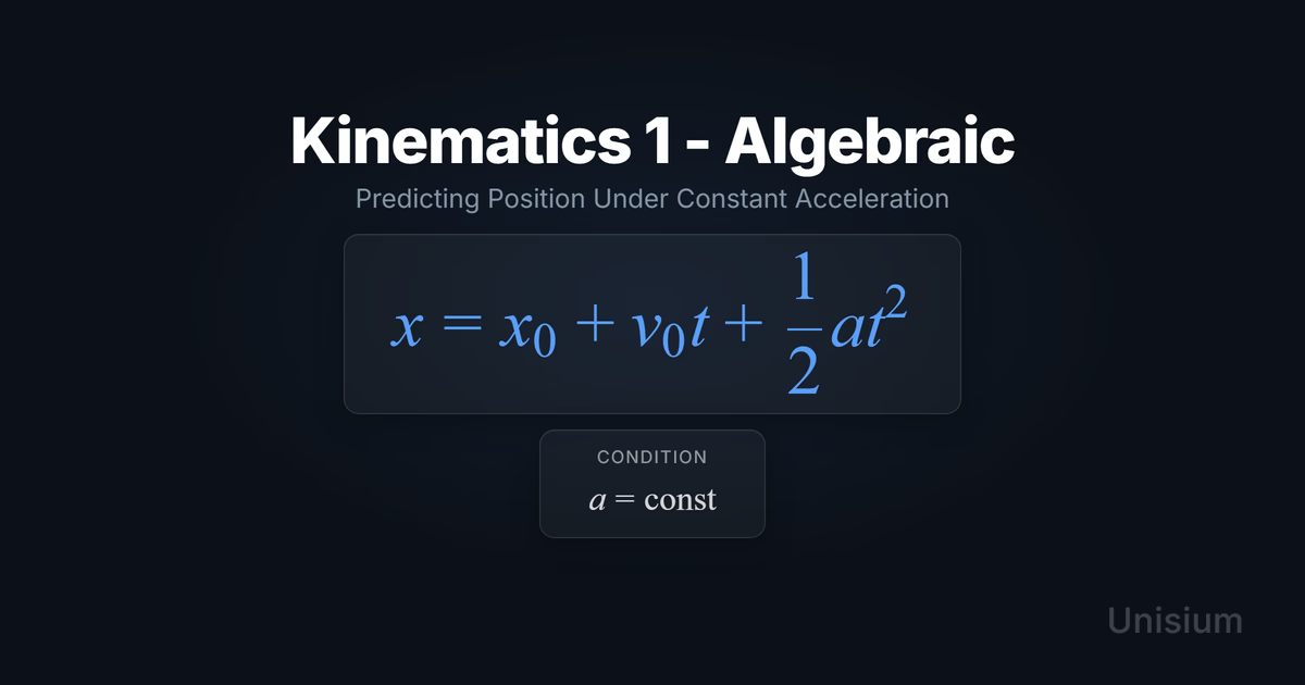
The Kinematics 1 - Algebraic principle states that for an object moving with constant acceleration, its final position is the sum of its initial position, the displacement due to initial velocity, and the displacement due to acceleration.

Mathematical Form

$x = x_0 + v_0 t + \frac{1}{2} a t^2$

Where:

• $x$ = final position (m)
• $x_0$ = initial position (m)
• $v_0$ = initial velocity (m/s)
• $a$ = constant acceleration (m/s²)
• $t$ = time interval (s)

Alternative Forms

In vector notation: $\vec{r} = \vec{r}_0 + \vec{v}_0 t + \frac{1}{2} \vec{a} t^2$

In 1D along the x-axis, this reduces to the scalar x-form.

---

Conditions of Applicability

Condition: $a=\mathrm{const}$ The acceleration vector must not change in magnitude or direction during the time interval.

Practical modeling notes

1. Constant Acceleration: The acceleration vector must not change in magnitude or direction during the time interval. Gravity near Earth’s surface ($g \approx 9.8$ m/s²) is a common example.
2. Inertial Frame: Standard kinematics applies in non-accelerating reference frames.
3. Point Particle: The object is treated as a particle or the motion refers to the center of mass of a non-rotating body.

When It Doesn’t Apply

• Variable Acceleration: If forces change (like air resistance increasing with speed, or a spring force changing with position), $a$ is not constant. You must use calculus ($\int v dt$) instead.
• Relativistic Speeds: At speeds close to the speed of light, Newtonian kinematics fails.

Want the complete framework behind this guide? Read Masterful Learning.

---

Common Misconceptions

The Average Velocity Trap

Students often try to use $x = vt$ (or $\Delta x = v t$) where $v$ is the final or initial velocity. This only works if acceleration is zero. For constant acceleration, you must use the full quadratic equation or the specific average velocity formula $\Delta x = \frac{1}{2}(v_0 + v)t$.

Sign Errors

Position, velocity, and acceleration are signed quantities in 1D. A common mistake is assuming $a$ is always negative (for gravity) or always positive. The sign depends entirely on your chosen coordinate system. If “up” is positive, gravity ($g$) creates negative acceleration ($a = -g$).

---

Elaborative Encoding

To truly learn this principle, don’t just memorize it. Use Elaborative Encoding to connect it to what you already know.

Within the Principle

1. Why is the time term squared ($t^2$) in the acceleration component?
2. How does the equation simplify if the object starts from rest ($v_0 = 0$)?

For the Principle

1. Which quantities must you know to predict position after time $t$ under constant acceleration?
2. How would timing a drop let you infer height, assuming constant acceleration? (No calculation—just describe the mapping.)

Between Principles

(Contrast with Kinematics 2): Kinematics 2 gives $v(t)=v_0+at$, while Kinematics 1 gives $x(t)$. Conceptually, how do you get from Kinematics 2 to Kinematics 1 (think “area under the $v$–$t$ graph”)?

Generate an Example

Create a scenario where an object has a positive velocity but a negative acceleration. How does the position change over time in this case?

---

Retrieval Practice

Test your explicit knowledge before applying it. See Retrieval Practice for the full method.

State the principle in words: _____Position as a function of time (constant acceleration)

Write the canonical equation: _____$x = x_0 + v_0 t + \frac{1}{2} a t^2$

State the canonical condition: _____$a=\mathrm{const}$

---

Worked Example

Use this worked example to practice Self-Explanation.

Problem: A cyclist is moving at $8.0$ m/s. They accelerate at a constant $0.80$ m/s² for $6.0$ seconds. How far do they travel during this interval?

Step 1: Verbal Decoding

Target: $\Delta x$
Given: $v_0$, $a$, $t$
Constraints: Constant acceleration, 1D motion

Step 2: Visual Decoding

Draw a 1D axis. Choose $+x$ in the direction of motion. Label $x_0 = 0$ at the start. Label $v_0$ and $a$ along $+x$. (So $v_0$ and $a$ are positive.)

Step 3: Physics Modeling

1. $\Delta x = v_0 t + \frac{1}{2} a t^2$

Step 4: Mathematical Procedures

1. $\Delta x = (8.0\,\mathrm{m/s})(6.0\,\mathrm{s}) + \frac{1}{2}(0.80\,\mathrm{m/s^2})(6.0\,\mathrm{s})^2$
2. $\Delta x = 48.0\,\mathrm{m} + 14.4\,\mathrm{m}$
3. $\underline{\Delta x = 62.4\,\mathrm{m}}$

Step 5: Reflection

• Units: Meters (matches distance).
• Magnitude: 62.4 m is reasonable for a bike accelerating for 6 seconds.
• Limiting Case: If $a=0$, distance would be $8.0 \times 6.0 = 48.0$ m. Since $a > 0$, the answer implies they went further than 48 m, which is correct.

Before moving on: Self-explain the model.

Physics model with explanation

Principle: Kinematics 1 - Algebraic. Conditions: The cyclist accelerates at a constant rate, justifying the constant acceleration model. Relevance: This equation directly links the known time interval and acceleration to the displacement. Description: We set the initial position to zero, so the displacement over the interval is $\Delta x$. Goal: Determine the final displacement to answer “how far”.

---

Solve a Problem

Apply what you’ve learned with Problem Solving.

Problem

A stone is thrown downward from a bridge with an initial speed of $5.0$ m/s. It hits the water $2.4$ seconds later. Air resistance is negligible. How high is the bridge? (Use $g = 9.8$ m/s²).

Show Solution

Step 1: Verbal Decoding

Target: $h$
Given: $v_0$, $t$, $g$
Constraints: Constant acceleration (free fall), negligible air resistance, vertical motion

Step 2: Visual Decoding

Draw a vertical y-axis. Choose $+y$ downward. Label $y_0 = 0$. Label $v_0$ downward (positive) and $a = g$ downward (positive). (So $v_0$ and $a$ are both positive.)

Step 3: Physics Modeling

1. $y = v_0 t + \frac{1}{2} g t^2$

Step 4: Mathematical Procedures

1. $y = (5.0\,\mathrm{m/s})(2.4\,\mathrm{s}) + \frac{1}{2}(9.8\,\mathrm{m/s^2})(2.4\,\mathrm{s})^2$
2. $y = 12\,\mathrm{m} + 28.224\,\mathrm{m}$
3. $y = 40.224\,\mathrm{m}$
4. $\underline{h = y \approx 40\,\mathrm{m}}$

Step 5: Reflection

• Units: Meters (height).
• Magnitude: 40m is a high bridge (approx 12-13 stories), plausible.
• Limiting Case: If thrown upward instead (negative $v_0$), the term $v_0 t$ would be negative, reducing the total distance for the same time, which makes sense.

---

Related Principles

• Classical Mechanics: The Complete Principle Map — see where this principle fits in the full subdomain.

Principle	Relation
Kinematics 2 (Velocity)	Finds final velocity given time: $v = v_0 + at$.
Kinematics 3 (Velocity-Position)	Finds velocity/position without time: $v^2 = v_0^2 + 2a\Delta x$.
Rotational Kinematics 1	Rotational analog: angular position vs time with constant angular acceleration.

---

Frequently Asked Questions

Can I use this equation if acceleration is zero?

Yes. If $a=0$, the term $\frac{1}{2}at^2$ vanishes, leaving $x = x_0 + v_0 t$. This perfectly matches the equation for constant velocity motion.

Why does the time squared term have a 1/2 factor?

The derivation from calculus shows that position is the integral of velocity ($v = v_0 + at$). Integrating $t$ with respect to $t$ gives $\frac{1}{2}t^2$. In geometric terms, this corresponds to the area of the triangle on a velocity-time graph representing the displacement due to changing velocity.

What if I don’t know the time?

If you are given displacement, initial velocity, and acceleration but not time, you might have to solve a quadratic equation for $t$. Alternatively, you can use Kinematics 3 ($v^2 = v_0^2 + 2a\Delta x$), which eliminates time entirely.

---

How This Fits in Unisium

Kinematics 1 is a foundational model in the Mechanics subdomain. It is often the first rigorous prediction tool students encounter. In Unisium, it serves as a bridge between simple arithmetic motion and the more complex dynamic laws of Newton. By mastering this through the Unisium Study System, you prepare your mind for more advanced relationship mappings like Work-Energy and Impulse-Momentum.

Related guides: Principle Structures · Self-Explanation · Retrieval Practice · Problem Solving

Ready to master Kinematics 1 - Algebraic? Start practicing with Unisium or explore the full learning framework in Masterful Learning.

Masterful Learning

The study system for physics, math, & programming that works: encoding, retrieval, self-explanation, principled problem solving, and more.

Read the book (opens in new tab) ISBN 979-8-2652-9642-9