Velocity-Position Relation: Kinematics 3
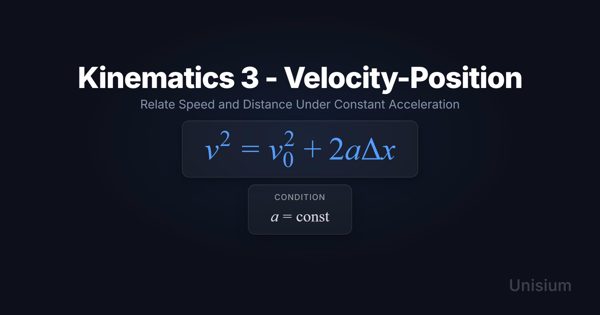
Kinematics 3 (Velocity-Position) relates an object’s velocity to its displacement under constant acceleration: . Use it when time is unknown or irrelevant, but you know (or want) , , , and .
On this page: The Principle · Conditions · Misconceptions · EE Questions · Retrieval Practice · Worked Example · Solve a Problem · FAQ
This relation is essential when time is unknown or irrelevant, such as finding how fast a car is moving after traveling a certain distance while braking at constant deceleration.
The Principle
Statement
When an object moves with constant acceleration, the square of its final velocity equals the square of its initial velocity plus twice the product of acceleration and displacement. This relation connects velocity and position without requiring the time variable.
Mathematical Form
Where:
- = final velocity (m/s)
- = initial velocity (m/s)
- = constant acceleration (m/s²)
- = displacement (m)
Alternative Forms
In different contexts, this appears as:
- Solving for displacement:
- Vector form:
Conditions of Applicability
Condition: Acceleration must remain constant throughout the interval. If acceleration varies, this relation does not hold.
Practical modeling notes
- For motion in a single dimension, the vector form reduces to the scalar form shown above.
- Sign conventions matter: choose a positive direction and stick with it throughout the problem.
- Displacement can be positive or negative depending on your coordinate choice.
When It Doesn’t Apply
- Varying acceleration: If acceleration changes during motion (e.g., air resistance that depends on speed), you cannot use this relation. Use calculus-based kinematics instead.
- Rotational motion: This principle applies only to translational motion. For rotation with constant angular acceleration, use the analogous rotational kinematic equation .
Want the complete framework behind this guide? Read Masterful Learning.
Common Misconceptions
Misconception 1: You can use this relation when acceleration varies
The truth: The derivation assumes constant acceleration. If acceleration changes, the relation breaks down because the average acceleration is not equal to the instantaneous acceleration at all points.
Why this matters: Using this equation for non-constant acceleration (like a car engine ramping up power) will give you incorrect velocities and lead to wrong predictions.
Misconception 2: and are speeds, not velocities
The truth: Both and are signed velocities (they can be positive or negative). Using magnitudes (speeds) without tracking direction will produce errors when motion reverses direction.
Why this matters: In problems where an object slows down, stops, and reverses (like a ball thrown upward), treating as always positive will give nonsensical results.
Misconception 3: This equation requires knowing the time
The truth: The power of this relation is that it eliminates time. It’s specifically useful when you don’t know (or don’t care about) the duration of motion—only initial/final velocities, acceleration, and displacement matter.
Why this matters: Students often reach for first, then struggle when time is not given. Recognizing when to use the time-independent form saves effort and avoids dead ends.
Elaborative Encoding
Use these questions to build deep understanding. (See Elaborative Encoding for the full method.)
Within the Principle
- Why does the equation contain and instead of just and ? What does squaring the velocity accomplish?
- What are the units on both sides of the equation, and why must they match?
For the Principle
- How do you decide whether to use this equation versus in a problem?
- If an object’s acceleration is negative (deceleration), how does that affect the sign and magnitude of each term in the equation?
Between Principles
- What is gained by eliminating time between Kinematics 2 () and Kinematics 1 () to obtain Kinematics 3, and what kind of problem does that make Kinematics 3 especially useful for?
Generate an Example
- Describe a real-world scenario where you would choose this equation over the other kinematic relations, and explain why time doesn’t matter in your example.
Retrieval Practice
Answer from memory, then click to reveal and check. (See Retrieval Practice for the full method.)
State the principle in words: _____The square of the final velocity equals the square of the initial velocity plus twice the product of acceleration and displacement.
Write the canonical equation: _____
State the canonical condition: _____
Worked Example
Use this worked example to practice Self-Explanation.
Problem
A car traveling at 25 m/s begins braking with a constant deceleration of 5.0 m/s². How far does the car travel before coming to rest?
Step 1: Verbal Decoding
Target:
Given: , ,
Constraints: Constant acceleration (deceleration), one-dimensional motion, car comes to rest
Step 2: Visual Decoding
Draw a 1D axis. Choose in the direction of initial motion (forward). Label pointing forward and at the stopping point. Label pointing backward (opposite to ). (So is positive and is negative.)
Step 3: Physics Modeling
Step 4: Mathematical Procedures
Step 5: Reflection
- Units: divided by gives ✓
- Magnitude: About 63 meters to stop from 25 m/s (~56 mph) with moderate braking is plausible.
- Limiting case: If (no braking), (car never stops), which makes sense.
Before moving on: self-explain the model
Try explaining Step 3 out loud (or in writing): why the velocity-position relation applies, what the signs mean, and how the equation encodes the braking scenario.
Physics model with explanation
Principle: We use the velocity-position kinematic relation because we know initial velocity, final velocity (zero), and acceleration, but time is not given or needed.
Conditions: The car brakes with constant deceleration, satisfying the constant acceleration condition.
Relevance: This equation directly connects velocity and displacement without requiring time, making it the most efficient choice for this problem.
Description: The car starts with forward velocity and decelerates at (negative because it opposes the motion). We want the displacement when the car reaches .
Goal: Solve for by rearranging the kinematic equation and substituting the known values.
Solve a Problem
Apply what you’ve learned with Problem Solving.
Problem
A ball is thrown upward from the ground with an initial velocity of 15 m/s. What is the ball’s velocity when it reaches a height of 8.0 m above the ground? (Use .)
Hint: Choose a coordinate system and be careful with signs for velocity and acceleration.
Show Solution
Step 1: Verbal Decoding
Target:
Given: , ,
Constraints: Constant acceleration (gravity), one-dimensional vertical motion
Step 2: Visual Decoding
Draw a 1D axis. Choose pointing upward. Label pointing upward at the launch point and at height 8.0 m. Label pointing downward (opposite to ). (So is positive, is negative, and could be positive or negative depending on whether the ball is rising or falling.)
Step 3: Physics Modeling
Step 4: Mathematical Procedures
Step 5: Reflection
- Units: under the square root gives ✓
- Magnitude: The ball slows from 15 m/s to about 8 m/s after rising 8 m, which is reasonable given gravity’s deceleration.
- Limiting case: If (no displacement), then , as expected.
Note on the two solutions
The equation gives two solutions () because the ball passes through 8.0 m twice—once going up (positive velocity) and once coming down (negative velocity). The problem context (ball is rising) selects the positive solution.
Related Principles
- Classical Mechanics: The Complete Principle Map — see where this principle fits in the full subdomain.
| Principle | Relationship to Kinematics 3 |
|---|---|
| Kinematics 1 | Relates position and time; combine it with Kinematics 2 to eliminate time and derive Kinematics 3 |
| Kinematics 2 | Relates velocity and time; pair it with Kinematics 1 when time is the variable you want to eliminate |
| Work–Energy Theorem | An energy-based alternative for finding velocity changes; equivalent when work equals kinetic energy change |
| Rotational Kinematics 3 | Rotational analog: angular velocity vs angular displacement. |
See Principle Structures for how to organize these relationships visually.
FAQ
What is the velocity-position kinematic relation?
It’s a formula that relates an object’s velocity to its displacement when acceleration is constant: . It allows you to solve for final velocity, initial velocity, acceleration, or displacement without knowing the time.
When does Kinematics 3 apply?
It applies when acceleration is constant throughout the motion. If acceleration varies (e.g., due to changing forces), you must use calculus-based methods or other kinematic approaches.
What’s the difference between Kinematics 3 and Kinematics 2?
Kinematics 2 () relates velocity to time, while Kinematics 3 () relates velocity to displacement. Use Kinematics 3 when you don’t know or don’t need the time; use Kinematics 2 when time is given or required.
What are the most common mistakes with Kinematics 3?
- Using it when acceleration is not constant.
- Forgetting to square the velocities (e.g., writing ).
- Mixing up speeds and velocities—signs matter for direction.
How do I know which kinematic equation to use?
List the known variables and the target variable. Then pick the equation that contains all four (and only four) of those variables. If you don’t know time and don’t need it, Kinematics 3 is usually the best choice.
Why does the equation have instead of ?
The squaring comes from integrating the acceleration over displacement (using the chain rule: ). This mathematical structure reflects how energy scales with the square of velocity.
Can I use this equation for circular motion?
Only if the acceleration is constant along the arc length, which is rare. For uniform circular motion, the acceleration is always perpendicular to velocity (centripetal), so the speed is constant and this equation is trivial ( with ).
How This Fits in Unisium
Unisium helps you master the velocity-position relation through targeted elaboration questions, retrieval prompts, worked examples with self-explanation scaffolds, and practice problems with immediate feedback. The system tracks which kinematic relations you confuse and surfaces comparisons to strengthen your discrimination between , , and .
Related guides: Principle Structures · Self-Explanation · Retrieval Practice · Problem Solving
Ready to master the velocity-position relation? Start practicing with Unisium or explore the full learning framework in Masterful Learning.

Masterful Learning
The study system for physics, math, & programming that works: retrieval, connection, explanation, problem solving, and more.
Ready to apply this strategy?
Join Unisium and start implementing these evidence-based learning techniques.
Start Learning with Unisium Read More GuidesWant the complete framework? This guide is from Masterful Learning.
Learn about the book →