Rotational Kinematics 1: Angular Position Under Constant Angular Acceleration

This principle is the rotational analog of the linear position-time equation. It applies to spinning wheels, rotating platforms, rolling objects, and any rigid body undergoing constant angular acceleration.

On this page: The Principle · Conditions · Misconceptions · EE Questions · Retrieval Practice · Worked Example · Solve a Problem · FAQ

---

The Principle

Statement

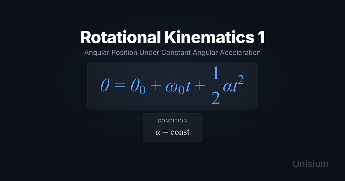
Rotational Kinematics 1 states that for angular motion with constant angular acceleration, its angular position at time $t$ is the sum of three contributions: the initial angular position, the angular displacement due to initial angular velocity, and the angular displacement due to angular acceleration.

Mathematical Form

$\theta = \theta_0 + \omega_0 t + \frac{1}{2} \alpha t^2$

Where:

• $\theta$ = final angular position (rad)
• $\theta_0$ = initial angular position (rad)
• $\omega_0$ = initial angular velocity (rad/s)
• $\alpha$ = constant angular acceleration (rad/s²)
• $t$ = time interval (s)

Alternative Forms

In terms of angular displacement $\Delta\theta = \theta - \theta_0$:

$\Delta\theta = \omega_0 t + \frac{1}{2} \alpha t^2$

This form is useful when you care about how far the object has rotated rather than its absolute angular position.

---

Conditions of Applicability

Condition: $\alpha=\mathrm{const}$ The angular acceleration must remain constant in magnitude and direction (sign) during the time interval.

Practical modeling notes

1. Rigid Body Assumption: The object must be rigid (no deformation) and rotate about a fixed axis. All points on the body have the same angular acceleration.
2. Inertial Frame: Standard rotational kinematics applies in non-accelerating reference frames.
3. Fixed Axis: The axis of rotation must not change direction during the motion. If the axis wobbles or precesses, this equation does not apply.

When It Doesn’t Apply

• Variable Angular Acceleration: If torque changes over time (such as a motor with changing power output, or friction that depends on angular speed), $\alpha$ is not constant. You must use calculus or numerical methods.

When You Need a Different Representation

These situations require more sophisticated models, not because $\alpha=\mathrm{const}$ fails, but because the simple 1-DOF description breaks down:

• Non-Rigid Bodies: If the object deforms significantly (like a spring unwinding), different parts have different angular accelerations.
• 3D Rotation: If the object tumbles or the axis changes direction, you need full 3D rotational dynamics with angular momentum vectors.

Want the complete framework behind this guide? Read Masterful Learning.

---

Common Misconceptions

Confusing Angular and Linear Kinematics

Students often mix up $\theta$, $\omega$, $\alpha$ with $x$, $v$, $a$. While the equations have identical structure, the quantities are fundamentally different: angular position is measured in radians, not meters. Always check units to avoid this error.

Forgetting the Zero-Point for Angular Position

Unlike position in linear motion, angular position $\theta_0$ can be arbitrary—you choose where $\theta = 0$ is. However, once chosen, you must remain consistent. A common mistake is resetting the zero-point mid-problem, which breaks the equation.

Assuming Constant Angular Velocity When It’s Not

If $\alpha \ne 0$, the angular velocity changes with time. Using $\theta = \omega t$ (valid only for constant $\omega$) instead of the full quadratic equation leads to incorrect predictions. The $\frac{1}{2} \alpha t^2$ term is often the dominant contribution in accelerating systems.

---

Elaborative Encoding

Use these questions to build deep understanding. (See Elaborative Encoding for the full method.)

Within the Principle

1. Why does the angular acceleration term include $t^2$ while the angular velocity term is linear in $t$?
2. If $\alpha$ and $\omega_0$ have opposite signs, what does the motion look like qualitatively? (Speeding up, slowing down, reversing?)

For the Principle

1. What three pieces of information must you know to predict angular position after time $t$ under constant angular acceleration?
2. If a wheel starts from rest and spins up under constant angular acceleration, which term in the equation contributes the most to $\theta$ after a long time?

Between Principles

How does this principle relate to the linear kinematics equation $x = x_0 + v_0 t + \frac{1}{2} a t^2$? What is the conceptual mapping between the two?

Generate an Example

Describe a real-world situation where a rotating object has constant angular acceleration. (Think about motors, spinning disks, or rolling objects.)

---

Retrieval Practice

Answer from memory, then click to reveal and check. (See Retrieval Practice for the full method.)

State the principle in words: _____For angular motion with constant angular acceleration, angular position at time t equals the initial angular position plus the displacement from initial angular velocity and the displacement from angular acceleration.

Write the canonical equation: _____$\theta = \theta_0 + \omega_0 t + \frac{1}{2} \alpha t^2$

State the canonical condition: _____$\alpha=\mathrm{const}$

---

Worked Example

Use this worked example to practice Self-Explanation.

Problem

A bicycle wheel starts from rest and accelerates at a constant angular acceleration of $2.5\,\mathrm{rad/s^2}$. What is the angular displacement after $4.0\,\mathrm{s}$?

Step 1: Verbal Decoding

Target: $\Delta\theta$ (angular displacement after 4.0 s)
Given: $\omega_0$, $\alpha$, $t$
Constraints: Constant angular acceleration; starts from rest

Step 2: Visual Decoding

Draw a wheel viewed from the side. Choose counterclockwise rotation as positive. Label $\omega_0 = 0$ and $\alpha > 0$. (So $\omega_0 = 0$ and $\alpha$ is positive.)

Step 3: Physics Modeling

1. $\Delta\theta = \omega_0 t + \frac{1}{2} \alpha t^2$

Step 4: Mathematical Procedures

1. $\Delta\theta = \omega_0 t + \frac{1}{2}\alpha t^2$
2. $\Delta\theta = \frac{1}{2}\alpha t^2 \quad (\omega_0 = 0)$
3. $\Delta\theta = \frac{1}{2} (2.5\,\mathrm{rad/s^2}) (4.0\,\mathrm{s})^2$
4. $\Delta\theta = \frac{1}{2} (2.5) (16)\,\mathrm{rad}$
5. $\underline{\Delta\theta = 20\,\mathrm{rad}}$

Step 5: Reflection

• Units: $\mathrm{rad/s^2} \cdot \mathrm{s^2} = \mathrm{rad}$ ✓
• Magnitude: 20 radians is about 3.2 full rotations, plausible for a wheel accelerating from rest over 4 seconds.
• Limiting case: If $t \to 0$, then $\Delta\theta \to 0$ (no rotation yet), which makes sense.

---

Before moving on: self-explain the model

Try explaining Step 3 out loud (or in writing): why Rotational Kinematics 1 applies, what each term represents physically, and how the equation encodes the situation.

Physics model with explanation (what “good” sounds like)

Principle: Rotational Kinematics 1 applies because we have a rigid body (the wheel) rotating about a fixed axis with constant angular acceleration.

Conditions: The problem states “constant angular acceleration,” satisfying $\alpha = \mathrm{const}$. The wheel is rigid and the axis is fixed.

Relevance: We need to predict angular position after a given time under constant angular acceleration, which is exactly what this principle does.

Description: The wheel starts from rest ($\omega_0 = 0$) at $t = 0$. We’re measuring angular displacement from the starting position. The only contribution is from the $\frac{1}{2} \alpha t^2$ term, which represents the angular displacement due to constant angular acceleration.

Goal: We’re solving for $\Delta\theta$ after $t = 4.0\,\mathrm{s}$. Since the wheel starts from rest, the displacement form simplifies to $\Delta\theta = \frac{1}{2} \alpha t^2$.

---

Solve a Problem

Apply what you’ve learned with Problem Solving.

Problem

A turntable is spinning at an initial angular velocity of $3.0\,\mathrm{rad/s}$ and slows down with a constant angular acceleration of $-0.50\,\mathrm{rad/s^2}$. What is the angular displacement after $5.0\,\mathrm{s}$?

Hint: The angular acceleration is negative, meaning the turntable is slowing down. Use the full equation with both $\omega_0 t$ and $\frac{1}{2} \alpha t^2$ terms.

Show Solution

Step 1: Verbal Decoding

Target: $\Delta\theta$ (angular displacement after 5.0 s)
Given: $\omega_0$, $\alpha$, $t$
Constraints: Constant angular acceleration; negative angular acceleration (slowing down)

Step 2: Visual Decoding

Draw a turntable viewed from above. Choose counterclockwise as positive. Label $\omega_0 > 0$ and $\alpha < 0$. (So $\omega_0$ is positive and $\alpha$ is negative.)

Step 3: Physics Modeling

1. $\Delta\theta = \omega_0 t + \frac{1}{2} \alpha t^2$

Step 4: Mathematical Procedures

1. $\Delta\theta = (3.0\,\mathrm{rad/s})(5.0\,\mathrm{s}) + \frac{1}{2} (-0.50\,\mathrm{rad/s^2}) (5.0\,\mathrm{s})^2$
2. $\Delta\theta = 15\,\mathrm{rad} + \frac{1}{2} (-0.50\,\mathrm{rad/s^2}) (25\,\mathrm{s^2})$
3. $\Delta\theta = 15\,\mathrm{rad} + \frac{1}{2} (-0.50)(25)\,\mathrm{rad}$
4. $\Delta\theta = 15\,\mathrm{rad} - 6.25\,\mathrm{rad}$
5. $\underline{\Delta\theta = 8.75\,\mathrm{rad}}$

Step 5: Reflection

• Units: $\mathrm{rad/s} \cdot \mathrm{s} = \mathrm{rad}$ and $\mathrm{rad/s^2} \cdot \mathrm{s^2} = \mathrm{rad}$ ✓
• Magnitude: About 1.4 full rotations is plausible for a turntable slowing down over 5 seconds from 3 rad/s.
• Limiting case: If $\alpha = 0$, we’d get $\Delta\theta = 15\,\mathrm{rad}$, so negative acceleration correctly reduces the displacement.

---

Related Principles

• Classical Mechanics: The Complete Principle Map — see where this principle fits in the full subdomain.

Principle	Relationship to Rotational Kinematics 1
Rotational Kinematics 2 ($\omega = \omega_0 + \alpha t$)	Gives angular velocity as a function of time; Rotational Kinematics 1 is derived by integrating this relation
Linear Kinematics 1 ($x = x_0 + v_0 t + \frac{1}{2} a t^2$)	Exact translational analog; same mathematical structure with angular quantities replacing linear ones
Rotational Kinematics 3 ($\omega^2 = \omega_0^2 + 2\alpha\Delta\theta$)	Eliminates time; useful when you know angular displacement and velocities but not time
Kinematics 1 (Position-Time)	Translation analog: linear position vs time with constant acceleration.

See Principle Structures for how to organize these relationships visually.

---

FAQ

What is Rotational Kinematics 1?

Rotational Kinematics 1 is the equation $\theta = \theta_0 + \omega_0 t + \frac{1}{2} \alpha t^2$ that predicts the angular position of a rotating rigid body as a function of time when angular acceleration is constant.

When does Rotational Kinematics 1 apply?

It applies when a rigid body rotates about a fixed axis with constant angular acceleration ($\alpha = \mathrm{const}$). Common examples include wheels spinning up or down under constant torque.

What’s the difference between Rotational Kinematics 1 and Linear Kinematics 1?

They have identical mathematical structure but describe different types of motion. Linear Kinematics 1 uses position ($x$), velocity ($v$), and acceleration ($a$), while Rotational Kinematics 1 uses angular position ($\theta$), angular velocity ($\omega$), and angular acceleration ($\alpha$). The equations are analogs of each other.

What are the most common mistakes with Rotational Kinematics 1?

The most common mistakes are (1) confusing angular and linear quantities, (2) forgetting the $\frac{1}{2} \alpha t^2$ term when acceleration is present, and (3) inconsistent sign conventions for $\omega_0$ and $\alpha$.

How do I know which form of Rotational Kinematics 1 to use?

If you need absolute angular position, use $\theta = \theta_0 + \omega_0 t + \frac{1}{2} \alpha t^2$. If you only care about how far the object has rotated (angular displacement), use $\Delta\theta = \omega_0 t + \frac{1}{2} \alpha t^2$. Both are equivalent—choose based on what the problem asks for.

---

Related Guides

• Principle Structures — Organize rotational kinematics in a hierarchical framework
• Self-Explanation — Learn to explain worked examples step by step
• Retrieval Practice — Make this principle instantly accessible
• Problem Solving — Apply principles systematically to new problems

---

How This Fits in Unisium

Unisium helps you master specific principles like Rotational Kinematics 1 through a four-stage learning system: elaborative encoding to build deep conceptual understanding, retrieval practice to make the principle instantly accessible, self-explanation to verify your understanding through worked examples, and problem solving to apply the principle to new situations. Each stage addresses a different bottleneck in learning, ensuring you don’t just memorize equations but truly understand when and how to use them.

Ready to master Rotational Kinematics 1? Start practicing with Unisium or explore the full learning framework in Masterful Learning.

Masterful Learning

The study system for physics, math, & programming that works: encoding, retrieval, self-explanation, principled problem solving, and more.

Read the book (opens in new tab) ISBN 979-8-2652-9642-9