Impulse-Momentum Theorem (Integral): General Time-Varying Forces
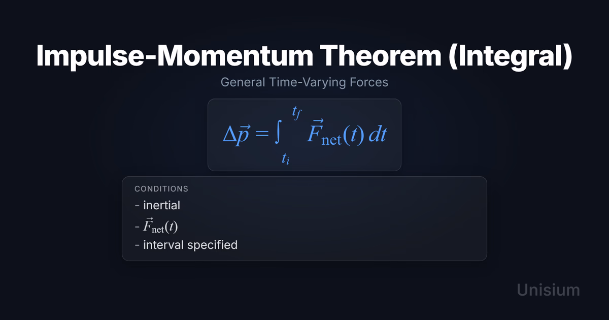
The Impulse-Momentum Theorem (Integral) states that the change in momentum of an object equals the integral of the net force over time: . It applies in an inertial frame. To use it, specify a time interval and model the net force as a function of time (constant is allowed).
This integral form is the most direct tool when you have a force–time model or force–time data over an interval. It handles arbitrary forces—making it a powerful tool for analyzing real-world momentum transfer where forces spike, decay, oscillate, or remain constant. The algebraic form is just this theorem rewritten using the definition of average force, but it’s only useful when you can compute or measure that average.
On this page: The Principle | Conditions | Misconceptions | EE Questions | Retrieval Practice | Worked Example | Solve a Problem | FAQ
The Principle
Statement
The Impulse-Momentum Theorem (Integral) states that the change in an object’s momentum over a time interval equals the time integral of the net force acting on it during that interval. This is the general calculus form that handles forces that may vary with time, arising directly from Newton’s second law by integrating over the interval from to .
Mathematical Form
Where:
- = change in momentum (kg·m/s, vector)
- = net force as a function of time (N, vector)
- = initial time (s)
- = final time (s)
- The integral represents the accumulated effect of force over time (units: N·s = kg·m/s)
Alternative Forms
In different contexts, this appears as:
- Component form (1D):
- Average-force form: , where
Conditions of Applicability
Condition: inertial; ; interval specified
This theorem applies universally in inertial frames. To use it for calculations, you need:
- Inertial reference frame: You must work in a frame that isn’t accelerating. Non-inertial frames (e.g., rotating carousel, accelerating rocket) require fictitious forces.
- Net force as a function of time: To compute the impulse, you need expressible as a function (or integrable data) over the interval.
- Time interval specified: You must define and to set the integration bounds (or solve for one of them).
Practical modeling notes
- Multiple objects: For systems of particles, apply to the total momentum: (only external forces contribute).
- Piecewise forces: If force is different in different time segments, break the integral into parts:
When the classical form needs modification
- Non-inertial frames: In an accelerating elevator or rotating platform, apparent forces appear. You must either switch to an inertial frame or include fictitious forces (Coriolis, centrifugal) in .
- Relativistic speeds: Near the speed of light, use relativistic momentum . The theorem still holds in relativistic form, but momentum is no longer simply .
When It’s Not Directly Usable
- Unknown impulse: If you can’t determine from force-time information, you need other constraints: momentum conservation (if net external impulse ), experimental measurement of impulse or average force, or additional dynamics information. The theorem still applies—you just can’t compute the impulse directly from .
If you’re deciding whether a problem should start with Conservation of Linear Momentum or with this theorem, see When to Use Momentum Conservation vs Impulse.
Want the complete framework behind this guide? Read Masterful Learning.
Common Misconceptions
Misconception 1: Impulse only applies to sudden collisions
The truth: The integral form applies to any net force over any duration—constant or time-dependent—whether it’s a 1 ms collision, a 10-second rocket burn, or a gradually increasing tension.
Why this matters: Students often reach for conservation of momentum when they should integrate a known force function. If you know , the impulse-momentum theorem gives you the momentum change directly without needing to know what happens to other objects.
Misconception 2: You need to know the position or trajectory to find momentum change
The truth: The impulse-momentum theorem bypasses position entirely. You only need force and time— depends on the time integral of force, not the path taken.
Why this matters: This makes the theorem powerful for situations where kinematic details are messy (e.g., a ball bouncing with spin, a car skidding with friction). You can find momentum change without solving differential equations for .
Misconception 3: The integral and algebraic forms are different theories
The truth: The algebraic form is just the integral theorem rewritten using the definition of average force: . They’re mathematically identical—one isn’t “more general.” The difference is practical: the integral form is useful when you know ; the algebraic form is useful when you know (or can measure) the average.
Why this matters: Don’t think you need a “special case” to use average force. You can always define it via the integral. The question is whether computing or measuring that average is easier than integrating directly.
Elaborative Encoding
Use these questions to build deep understanding. (See Elaborative Encoding for the full method.)
Within the Principle
- Why do force and time both appear in the integral, and what physical quantity does represent in terms of units?
- The equation is a vector equation—what does it mean to integrate a vector function over time?
For the Principle
- How do you decide whether to use the integral form versus the algebraic form () in a collision problem?
- If you know the force function but the problem asks for final velocity, what additional information do you need to solve?
Between Principles
- How does the impulse-momentum theorem (integral) relate to Newton’s second law ?
Generate an Example
- Describe a situation where you have a force-vs-time model or data, so integrating (or computing from the integral) is the natural approach—specify the object, the force function, and the time interval.
Retrieval Practice
Answer from memory, then click to reveal and check. (See Retrieval Practice for the full method.)
State the principle in words: _____The change in momentum of an object equals the time integral of the net force acting on it over the specified interval.
Write the canonical equation: _____
State the canonical condition: _____
Worked Example
Use this worked example to practice Self-Explanation.
Problem
A 0.50 kg hockey puck is initially at rest on frictionless ice. A time-varying horizontal force is applied in the direction according to starting at and ending at . Find the puck’s final speed.
Step 1: Verbal Decoding
Target: (final speed)
Given: , , , ,
Constraints: Initially at rest, frictionless horizontal surface, force varies linearly with time over a known interval
Step 2: Visual Decoding
Draw a 1D axis. Choose to the right. Label in the direction. Label and on the axis with signs. (So is zero and is positive.)
Step 3: Physics Modeling
Step 4: Mathematical Procedures
Step 5: Reflection
- Units: The integral gives N·s = kg·m/s (momentum units). Final velocity is m/s. ✓
- Magnitude: 48 m/s (~170 km/h) is fast but plausible for a light puck under strong acceleration over 2 seconds.
- Limiting case: If the force were zero or the time interval zero, and , as expected.
Before moving on: self-explain the model
Try explaining Step 3 out loud (or in writing): why the chosen principle applies, what the diagram implies, and how the equations encode the situation.
Physics model with explanation (what “good” sounds like)
Principle: The impulse-momentum theorem (integral) connects the time integral of net force to the change in momentum. This is the correct tool when you use force-over-time information to predict momentum change.
Conditions: We’re on Earth’s surface (inertial frame to good approximation), the force is given as an explicit function , and we have a specified time interval . All three conditions are met.
Relevance: The force is given as an explicit function . The integral form directly computes the impulse without needing to first calculate the average force.
Description: The puck starts at rest, so . The force ramps up from 0 to 24 N over 2 seconds. The integral computes the total impulse (area under the vs. graph). That impulse equals the momentum change. Since mass is constant and , all the momentum goes into .
Goal: We want final speed. The integral gives . Dividing by mass yields .
Solve a Problem
Apply what you’ve learned with Problem Solving.
Problem
A 1200 kg car is traveling at 15 m/s when the driver applies the brakes. The braking force (in the direction opposite to motion) varies with time as for the first 3.0 seconds, then drops to zero. Assume the road is horizontal and ignore air resistance. Find the car’s speed after 3.0 seconds. (Work in 1D; choose the initial direction of motion as positive.)
Hint: The force opposes motion, so it’s negative in your chosen coordinate system.
Show Solution
Step 1: Verbal Decoding
Target:
Given: , , , ,
Constraints: 1D horizontal motion, braking force opposite , constant mass, negligible air resistance
Step 2: Visual Decoding
Draw a 1D axis. Choose in the direction of the initial motion. Label as positive. Label in the negative direction. (So is positive and the impulse is negative.)
Step 3: Physics Modeling
Step 4: Mathematical Procedures
Step 5: Reflection
- Units: Integral gives N·s = kg·m/s; final answer is m/s. ✓
- Magnitude: Car slowed from 15 m/s to 6 m/s (lost 9 m/s) in 3 seconds under increasing braking force—reasonable deceleration.
- Limiting case: If braking time were zero or force were zero, and the car would maintain , as expected.
Related Principles
- Classical Mechanics: The Complete Principle Map — see where this principle fits in the full subdomain.
| Principle | Relationship to Impulse-Momentum Theorem (Integral) |
|---|---|
| Newton’s Second Law | The impulse-momentum theorem is derived by integrating over time—it’s the time-integrated form of Newton’s second law. |
| Impulse-Momentum Theorem (Algebraic) | The algebraic form is the integral form rewritten using . Same physics; different inputs. Use integral form when you know ; use algebraic when you know . |
| Conservation of Linear Momentum | When , the impulse is zero, so —momentum is conserved. The impulse-momentum theorem explains when and why momentum conservation holds. |
See Principle Structures for how to organize these relationships visually.
FAQ
What is the Impulse-Momentum Theorem (Integral)?
The Impulse-Momentum Theorem (Integral) states that the change in an object’s momentum equals the time integral of the net force: . It applies in an inertial frame; to use it you need a force model (which may be constant or time-dependent) and an interval.
When does the integral form apply versus the algebraic form?
Both forms are mathematically equivalent—the algebraic form uses the definition of average force. The choice is practical: use the integral form when you know or have force-vs-time data you can integrate. Use the algebraic form when you know (or can measure/estimate) directly, including constant-force cases where .
What’s the difference between impulse and momentum?
Momentum is a property of a moving object. Impulse is the accumulated effect of force over time—it’s what changes momentum. Think: momentum is like “motion bank account,” impulse is a “transaction.”
What are the most common mistakes with the integral form?
- Forgetting the sign/direction: Force and momentum are vectors. If force opposes motion, it’s negative in your coordinate system.
- Confusing with : Impulse integrates force over time, not distance (that’s work).
- Using the algebraic form with an assumed : The real error is inventing or guessing an average force (e.g., using midpoint force) when you can’t justify it. If you have data, compute from the integral or integrate directly.
How do I know which form of the impulse-momentum theorem to use?
- Known function: Use the integral form.
- Known average force or constant force: Use the algebraic form .
- Unknown forces, isolated system: Use conservation of momentum (total external impulse is zero).
- Collision with known velocities: Often easier to use conservation of momentum unless you need to find forces.
Related Guides
- Principle Structures — Organize the impulse-momentum theorem in a hierarchical framework
- Self-Explanation — Learn to explain worked examples step by step
- Retrieval Practice — Make this principle instantly accessible
- Problem Solving — Apply principles systematically to new problems
How This Fits in Unisium
Mastering the Impulse-Momentum Theorem (Integral) means more than memorizing the formula—it requires building deep connections (elaborative encoding), retrieving it effortlessly (retrieval practice), explaining why it works (self-explanation), and applying it to varied problems (problem solving). The Unisium Study System integrates these four strategies into every learning session, helping you move from formula recognition to confident application in collisions, rocket propulsion, and any scenario with time-varying forces.
Ready to master the Impulse-Momentum Theorem (Integral)? Start practicing with Unisium or explore the full learning framework in Masterful Learning.

Masterful Learning
The study system for physics, math, & programming that works: retrieval, connection, explanation, problem solving, and more.
Ready to apply this strategy?
Join Unisium and start implementing these evidence-based learning techniques.
Start Learning with Unisium Read More GuidesWant the complete framework? This guide is from Masterful Learning.
Learn about the book →