Taylor Polynomial Definition: Approximating Functions with Polynomials

On this page: The Principle | Conditions | Misconceptions | EE Questions | Retrieval Practice | Worked Example | Solve a Problem | FAQ

---

The Principle

Statement

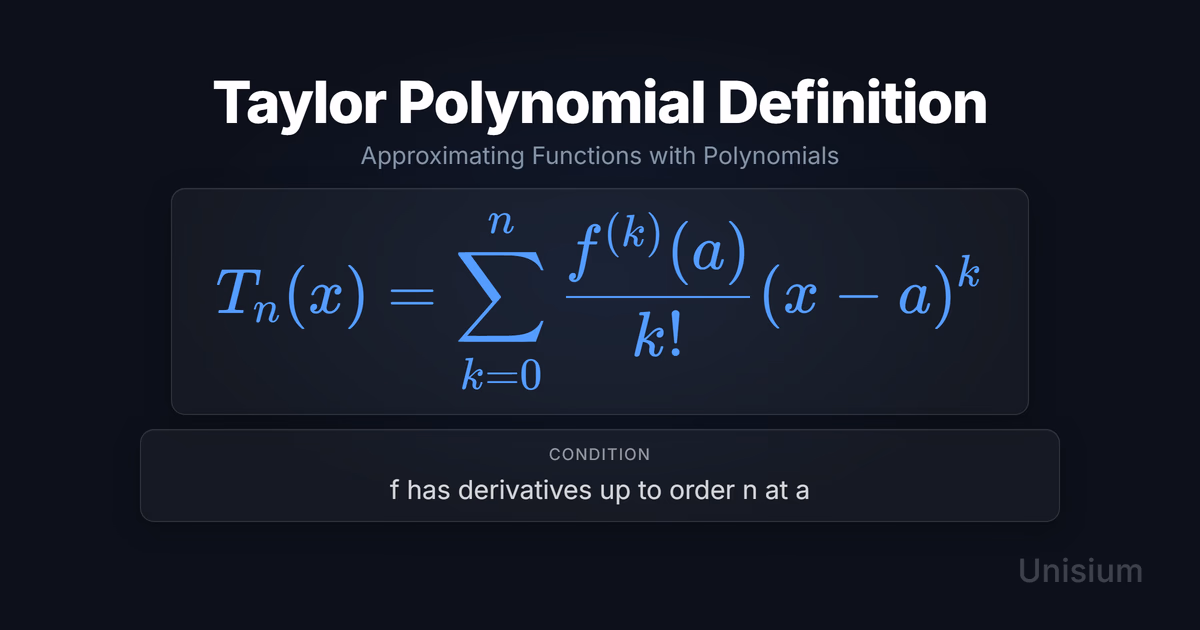
The Taylor polynomial definition says that for a function $f$ with derivatives up to order $n$ at $a$, the nth Taylor polynomial at $a$ is the polynomial $T_n(x) = \sum_{k=0}^n \frac{f^{(k)}(a)}{k!}(x-a)^k$, where $f^{(0)}(a) = f(a)$ by convention. $T_n$ is the unique polynomial of degree at most $n$ satisfying $T_n^{(k)}(a) = f^{(k)}(a)$ for every $k = 0, 1, \ldots, n$.

Mathematical Form

$T_n(x) = \sum_{k=0}^n \frac{f^{(k)}(a)}{k!}(x-a)^k$

Where:

• $n$ = the degree of the polynomial (a non-negative integer)
• $x$ = the input variable
• $a$ = the center (the point at which the polynomial is built)
• $f^{(k)}(a)$ = the $k$th derivative of $f$ evaluated at $a$ (with $f^{(0)}(a) = f(a)$)
• $k!$ = $k$ factorial, with $0! = 1$

Alternative Forms

In different contexts, this appears as:

• Explicit terms (degree 3, center $a$): $T_3(x) = f(a) + f'(a)(x-a) + \frac{f''(a)}{2}(x-a)^2 + \frac{f'''(a)}{6}(x-a)^3$
• Maclaurin polynomial ($a = 0$): $T_n(x) = \sum_{k=0}^n \frac{f^{(k)}(0)}{k!}x^k$

---

Conditions of Applicability

Condition: f has derivatives up to order n at a

Practical modeling notes

• “Has derivatives up to order $n$ at $a$” means $f'(a),\, f''(a),\, \ldots,\, f^{(n)}(a)$ all exist as finite real numbers. For elementary functions ($e^x$, $\sin x$, $\cos x$, polynomials), all derivatives exist everywhere, so the condition holds for any $n$ and any $a$.
• The $\frac{1}{k!}$ factor is not optional—it is the exact correction that makes $T_n^{(k)}(a) = f^{(k)}(a)$. Omitting it produces a polynomial whose derivatives at $a$ do not match $f$‘s.
• Choose $a$ at a value where evaluation is easy: $a = 0$ (the Maclaurin case) often gives the simplest arithmetic for $e^x$, $\sin x$, and $\cos x$.
• $T_n(x)$ is the definition of the polynomial and says nothing about how accurate the approximation is away from $a$. How quickly the error grows with $|x - a|$ is determined by the Taylor remainder theorem, which is a separate result.

When It Doesn’t Apply

• Insufficient differentiability: If $f$ does not have an $n$th derivative at $a$, the $n$th Taylor polynomial at $a$ is not defined. For example, $|x|$ is not differentiable at $x = 0$, so $T_1(x)$ at $a = 0$ does not exist for $|x|$.

Want the complete framework behind this guide? Read Masterful Learning.

---

Common Misconceptions

Misconception 1: $T_n(x)$ equals $f(x)$ on its entire domain

The truth: $T_n(x)$ agrees with $f$ and all its derivatives up to order $n$ at $a$, but $T_n(x) \ne f(x)$ in general. The degree-1 polynomial $T_1(x) = 1 + x$ agrees with $e^x$ and its first derivative at $x = 0$, but their values diverge for any $x \ne 0$.

Why this matters: Treating $T_n$ as equal to $f$ leads to errors when computing $f$ far from $a$ or when identifying when an approximation loses reliability.

Misconception 2: The $k!$ in the denominator is just a scaling convention

The truth: $\frac{d^k}{dx^k}(x-a)^k = k!$, so dividing by $k!$ is exactly what makes the $k$th derivative of $T_n$ at $a$ equal $f^{(k)}(a)$. The factorial is not cosmetic—it is the mechanism behind the defining matching property.

Why this matters: Students who drop or misplace the $k!$ produce polynomials whose derivatives at $a$ do not match $f$‘s, violating the definition and giving incorrect coefficients.

---

Elaborative Encoding

Use these questions to build deep understanding. (See Elaborative Encoding for the full method.)

Within the Principle

• In $T_n(x) = \sum_{k=0}^n \frac{f^{(k)}(a)}{k!}(x-a)^k$, what does each factor in the $k$th term ($f^{(k)}(a)$, $k!$, and $(x-a)^k$) contribute? Why must all three factors be present?
• What is the value of $T_n(a)$? What is $T_n'(a)$? What does this reveal about what “matching at $a$” means geometrically and analytically?

For the Principle

• Given a function $f$ and a target degree $n$, how do you identify the center $a$ that makes the derivatives easiest to evaluate?
• Suppose $f$ is three-times differentiable at $a$ but not four-times differentiable. For which values of $n$ can you build $T_n(x)$ there, and for which does the definition fail?

Between Principles

• The tangent line equation at $a$ is $y = f(a) + f'(a)(x-a)$. How does $T_1(x)$ compare to it? What does $T_n$ for $n \ge 2$ capture that the tangent line cannot?

Generate an Example

• Describe a function $f$ and a center $a$ where the Taylor polynomial $T_2(x)$ is exactly equal to $f(x)$ for all $x$. What does this say about functions that are themselves polynomials of low degree?

---

Retrieval Practice

Answer from memory, then click to reveal and check. (See Retrieval Practice for the full method.)

State the principle in words: _____The nth Taylor polynomial of f at a is the unique polynomial of degree at most n matching f and its first n derivatives at a, given by the sum from k=0 to n of f^(k)(a) over k! times (x-a)^k.

Write the canonical equation: _____$T_n(x)=\sum_{k=0}^n \frac{f^{(k)}(a)}{k!}(x-a)^k$

State the canonical condition: _____f has derivatives up to order n at a

---

Worked Example

Use this worked example to practice Self-Explanation.

Problem

Let $f(x) = e^x$. Find the Taylor polynomial $T_3(x)$ at $a = 0$.

Step 1: Verbal Decoding

Target: $T_3(x)$, the degree-3 Taylor polynomial of $f$ at $a = 0$
Given: $f$, $a$, $n$
Constraints: $f(x) = e^x$; $a = 0$; $n = 3$; $e^x$ is differentiable everywhere

Step 2: Visual Decoding

Mark $a = 0$ on the $x$-axis. $T_3$ will touch $e^x$ at $x = 0$ and match its slope, curvature, and third-derivative rate there; it diverges from $e^x$ as $|x|$ grows. (The polynomial is a cubic that closely tracks the exponential only near $x = 0$.)

Step 3: Mathematical Modeling

1. $T_3(x) = \sum_{k=0}^3 \frac{f^{(k)}(0)}{k!}x^k$

Step 4: Mathematical Procedures

1. $f^{(0)}(0)=1,\quad f^{(1)}(0)=1,\quad f^{(2)}(0)=1,\quad f^{(3)}(0)=1$
2. $T_3(x) = \frac{1}{0!} + \frac{1}{1!}x + \frac{1}{2!}x^2 + \frac{1}{3!}x^3$
3. $\underline{T_3(x) = 1 + x + \frac{x^2}{2} + \frac{x^3}{6}}$

Step 5: Reflection

• Verification: $T_3(0) = 1 = e^0$ ✓; $T_3'(0) = 1 = (e^x)'|_{x=0}$ ✓; $T_3''(0) = 1 = (e^x)''|_{x=0}$ ✓.
• Graphical meaning: Near $x = 0$, $T_3(x)$ tracks $e^x$ closely; for $|x| > 2$ the cubic departs noticeably.
• Limiting case: At $n = 1$, $T_1(x) = 1 + x$—the tangent line to $e^x$ at $a = 0$.

---

Before moving on: self-explain the model

Try explaining Step 3 out loud (or in writing): why the definition uses $f^{(k)}(0)/k!$ rather than $f^{(k)}(0)$ alone, why all four coefficients equal $1$ for $e^x$, and how $T_3$ would change if the center were $a = 1$ instead of $a = 0$.

Mathematical model with explanation

Principle: Taylor polynomial definition — $T_n(x) = \sum_{k=0}^n \frac{f^{(k)}(a)}{k!}(x-a)^k$ instantiated with $n = 3$, $a = 0$.

Conditions: $e^x$ has derivatives of all orders everywhere, so the condition is satisfied for any $n$ and any $a$.

Relevance: Every derivative of $e^x$ equals $e^x$, so every $f^{(k)}(0) = e^0 = 1$, making the coefficient evaluation trivial.

Description: Substitute $f^{(k)}(0) = 1$ for $k = 0, 1, 2, 3$ and simplify $1/k!$ for each term.

Goal: Produce the explicit cubic $1 + x + \frac{x^2}{2} + \frac{x^3}{6}$, which matches $e^x$ and its first three derivatives at $x = 0$.

---

Solve a Problem

Apply what you’ve learned with Problem Solving.

Problem

Let $f(x) = \cos x$. Find the Taylor polynomial $T_4(x)$ at $a = 0$.

Hint (if needed): Compute $f^{(k)}(0)$ for $k = 0, 1, 2, 3, 4$ by cycling through the known derivatives of $\cos x$.

Show Solution

Step 1: Verbal Decoding

Target: $T_4(x)$, the degree-4 Taylor polynomial of $\cos x$ at $a = 0$
Given: $f$, $a$, $n$
Constraints: $f(x) = \cos x$; $a = 0$; $n = 4$; $\cos x$ is differentiable everywhere

Step 2: Visual Decoding

Mark $a = 0$ on the $x$-axis. Derivatives of $\cos x$ cycle: $\cos x \to -\sin x \to -\cos x \to \sin x \to \cos x$. At $x = 0$ the pattern gives values $1, 0, -1, 0, 1$ for orders $0$ through $4$. (Only even-order terms survive because $\sin(0) = 0$.)

Step 3: Mathematical Modeling

1. $T_4(x) = \sum_{k=0}^4 \frac{f^{(k)}(0)}{k!}x^k$

Step 4: Mathematical Procedures

1. $f^{(0)}(0)=1,\quad f^{(2)}(0)=-1,\quad f^{(4)}(0)=1$
2. $f^{(1)}(0)=0,\quad f^{(3)}(0)=0$
3. $T_4(x) = \frac{1}{0!} + \frac{0}{1!}x + \frac{-1}{2!}x^2 + \frac{0}{3!}x^3 + \frac{1}{4!}x^4$
4. $\underline{T_4(x) = 1 - \frac{x^2}{2} + \frac{x^4}{24}}$

Step 5: Reflection

• Verification: $T_4(0) = 1 = \cos(0)$ ✓; $T_4''(0) = -1 = (\cos x)''|_{x=0}$ ✓.
• Graphical meaning: Odd-degree terms vanish because $\cos x$ is even; $T_4$ is a polynomial in $x^2$ only, symmetric about the $y$-axis.
• Domain check: The zero coefficients at $k = 1, 3$ are correct—$f'(0) = -\sin(0) = 0$ and $f'''(0) = \sin(0) = 0$, not missing terms.

---

Related Principles

Principle	Relationship to Taylor Polynomial Definition
Derivative at a point ($f'(a) = \lim_{h \to 0}\frac{f(a+h)-f(a)}{h}$)	Prerequisite — each $f^{(k)}(a)$ is a derivative value; without the ability to evaluate derivatives at $a$, no Taylor polynomial can be built
Linear approximation ($f(x) \approx f(a) + f'(a)(x-a)$)	The degree-1 case: $T_1(x) = f(a) + f'(a)(x-a)$ is the linear approximation, matching only value and slope
Tangent line equation ($y - f(a) = f'(a)(x-a)$)	$T_1(x)$ is exactly the tangent line rewritten; the Taylor polynomial generalizes the tangent line to higher-order polynomial fits

See Principle Structures for how these relationships fit hierarchically in calculus.

---

FAQ

What is the Taylor polynomial definition?

The Taylor polynomial of degree $n$ at center $a$ is $T_n(x) = \sum_{k=0}^n \frac{f^{(k)}(a)}{k!}(x-a)^k$. It is the unique polynomial of degree at most $n$ that matches $f$ and each of its first $n$ derivatives at $a$. The condition is that $f$ must have derivatives up to order $n$ at $a$.

What does “f has derivatives up to order n at a” mean?

It means $f'(a),\, f''(a),\, \ldots,\, f^{(n)}(a)$ all exist as finite real numbers at exactly the point $x = a$. For $e^x$, $\sin x$, $\cos x$, and polynomials, all derivatives exist everywhere, so the condition holds for any $n$ at any $a$.

What is a Maclaurin polynomial?

A Maclaurin polynomial is the Taylor polynomial built at the center $a = 0$: $T_n(x) = \sum_{k=0}^n \frac{f^{(k)}(0)}{k!}x^k$. The name honors Colin Maclaurin, but it is just the $a = 0$ special case of the Taylor polynomial definition.

Why is the coefficient $\frac{f^{(k)}(a)}{k!}$ and not simply $f^{(k)}(a)$?

Differentiating $(x-a)^k$ exactly $k$ times yields $k!$, so the $k$th derivative of $c_k(x-a)^k$ at $a$ is $c_k \cdot k!$. Setting $c_k = \frac{f^{(k)}(a)}{k!}$ makes $T_n^{(k)}(a) = f^{(k)}(a)$ exactly. The factorial is the mechanism, not decoration.

How does the Taylor polynomial relate to the Taylor series?

The Taylor series of $f$ at $a$ is the infinite sum $\sum_{k=0}^{\infty} \frac{f^{(k)}(a)}{k!}(x-a)^k$ (requiring all derivatives to exist at $a$). The $n$th Taylor polynomial $T_n$ is the partial sum of the series through degree $n$. Whether the series converges to $f$ for a given $x$ is a separate question addressed by the Taylor remainder theorem and the radius of convergence.

---

Related Guides

• Principle Structures — Organize the Taylor polynomial in a hierarchical framework with the derivative definition and approximation principles
• Linear Approximation — The first-order Taylor polynomial is the nearest downstream special case and the first approximation model most students use
• Self-Explanation — Practice explaining why each term carries $f^{(k)}(a)/k!$ as you work through examples
• Retrieval Practice — Make the equation and condition accessible under exam pressure
• Problem Solving — Apply the Five-Step Strategy to Taylor polynomial problems systematically

---

How This Fits in Unisium

Unisium structures the Taylor polynomial definition as a representational principle: the equation $T_n(x) = \sum_{k=0}^n \frac{f^{(k)}(a)}{k!}(x-a)^k$ is the model you instantiate by evaluating derivatives at $a$, and expanding the sum is the procedure. The platform surfaces this principle through elaborative encoding exercises, retrieval cues, and worked problem sets so you build the habit of identifying $f$, $a$, and $n$ before computing any coefficient—rather than trying to reconstruct the formula from scratch under pressure. Because the Taylor polynomial reappears in local approximation, Taylor series convergence, differential equations, and numerical methods, mastering its definition here compounds into fluency across the rest of calculus.

Ready to master the Taylor polynomial definition? Start practicing with Unisium or explore the full learning framework in Masterful Learning.

Masterful Learning

The study system for physics, math, & programming that works: retrieval, connection, explanation, problem solving, and more.

Read the book (opens in new tab) ISBN 979-8-2652-9642-9